
clusterMaker: Creating and Visualizing Cytoscape Clusters
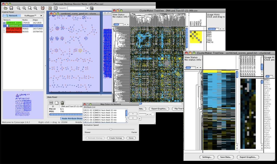
Figure 1. clusterMaker in action. In this screenshot, the expression data in the sampleData file galFiltered.cys has been clustered using the hierarchical method and displayed as a heatmap with associated dendrogram. The groups created by clustering are shown on the network.
In addition to this documentation, there are four tutorials available on the Open Tutorials web site under the "Cytoscape Tutorials" section. The first tutorial: Cluster Maker covers some of the basic features and uses of clusterMaker. The other three tutorials describe the steps necessary to reproduce the scenarios described in the BMC Bioinformatics publication: "clusterMaker: A Multi-algorithm Clustering Plugin for Cytoscape", currently submitted. This publication had three scenarios:
- BMC Bioinformatics Scenario 1: Gene expression analysis in a network context.
- BMC Bioinformatics Scenario 2: Finding complexes in proteomic and genetic interaction data.
- BMC Bioinformatics Scenario 3: Functional annotation by clustering protein similarity networks.
Contents
- Installation
- Starting ClusterMaker
- Attribute Cluster Algorithms
- Network Cluster Algorithms
- Filtering Clusters
- Visualizing Results
- Interaction
- Commands
- Acknowledgements
- References
1. Installation
clusterMaker is available through the Cytoscape plugin manager or by downloading the source directly from the Cytoscape svn repository (see Cytoscape Subversion Server information, or browse the csplugins/ucsf/scooter/clusterMaker sources). To download clusterMaker using the plugin manager, you must be running Cytoscape 2.8.2 or newer. clusterMaker is available in the Analysis group of plugins. To install it, bring up the Manage Plugins dialog (Plugins→Manage Plugins) and select Analysis under Available for Install. Select clusterMaker and click the Install button.
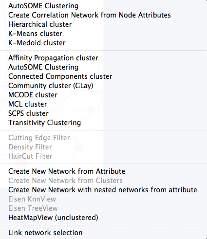
Figure 2. clusterMaker plugin menu.
2. Starting ClusterMaker
Once clusterMaker is installed, it will install a new Cluster menu hierarchy under the Plugins main menu. Each of the supported clustering algorithms appears as a separate menu item underneath the Cluster menu. To cluster your data, simply select Plugins→Cluster→algorithm where algorithm is the clustering algorithm you wish to use (see Figure 2). This will bring up the settings dialog for the selected algorithm (see below).
The Cluster menu also contains a subset of the visualization options, including showing a heat map of the data (without clustering), and options appropriate for displaying Hierarchical or k-Means clusters if either of those methods had been performed on the current network. Because information about clusters is saved in Cytoscape attributes, the Eisen TreeView and Eisen KnnView options will be available in a session that was saved after clustering.
There are two different types of clustering algorithms supported by clusterMaker:
- attribute clustering: a list of node attributes or a single edge attribute is chosen to perform the clustering. The normal visualization is some kind of heat map where the rows correspond to the nodes in the network. Selection of a row selects the corresponding node in the network. If an edge attribute is chosen, the columns also correspond to the nodes in the network and selection of cell in the heat map selects an edge in the network.
- network clustering: an edge attribute is chosen to partition the network. The normal visualization is to create a new network from the clusters.
3. Attribute Cluster Algorithms
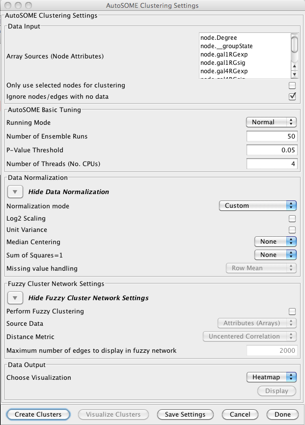
Figure 3. clusterMaker AutoSOME cluster dialog.
3.1 AutoSOME
AutoSOME clustering is the one cluster algorithm that functions both as an attribute cluster algorithm as well as a network cluster algorithm. The AutoSOME algorithm revolves around the use of a Self-Organizing Map (SOM). Unsupervised training of the SOM produces a low-dimensional reprentation of input space. In AutoSOME, that dimensionally reduced spaced is compresed into a 2D representation of similarities between neighboring nodes across the SOM network. These nodes are further distorted in 2D space based on their density of similarity to each other.Afterwards, a minimum spanning tree is built from rescaled node coordinates. Monte-Carlo sampling is used to calculate p-values for all edges in the tree. Edges below an inputed P-value Threshold are then deleted, leaving behind the clustering results. AutoSOME clustering may be repeated multiple times to minimize stochastic-based output variation. The clustering results stabilize at maximum quality with an increasing Number of Ensemble Runs, which is one of the input parameters. Statistically, 25-50 ensemble runs is enough to generate stable clustering.
Data Input
- Array Sources (Node Attributes):
- This area contains the list of all numeric node and edge attributes that can be used for hierarchical clustering. At least one edge attribute or one or more node attributes must be selected to perform the clustering. If an edge attribute is selected, the resulting matrix will be symmetric across the diagonal with nodes on both columns and rows. If multiple node attributes are selected, the attributes will define columns and the nodes will be the rows.
- Only use selected nodes/edges for cluster:
- Under certain circumstances, it may be desirable to cluster only a subset of the nodes in the network. Checking this box limits all of the clustering calculations and results to the currently selected nodes or edges.
- Ignore nodes/edges with no data:
- A common use of clusterMaker is to map expression data onto a pathway or protein-protein interaction network. Often the expression data will not cover all of the nodes in the network, so the resulting dendrogram will have a number of "holes" that might make interpretation more difficult. If this box is checked, only nodes that have values for at least one of the attributes will be included in the matrix.
AutoSOME Basic Tuning
- Runing Mode:
-
Changing the AutoSOME Running Mode will change the number of iterations used for training and the resolution
of the cartogram (see the paper for a full description of these parameters).
- Normal
- This setting has less cluster resolving power than Precision mode, but is ~4X faster. In addition, empirical experiments indicate that the two settings often result in comparable performance.
- Precision
- This setting
- Speed
- Speed mode has the least precision, but is very fast and may be desired for a first pass.
- Number of Ensemble Runs:
- Number of times clustering is repeated to stabilize final results. 25-50 ensemble runs is usually enough.
- P-Value Threshold:
- Threshold determining which edges are deleted in minimun spanning trees generated from Monte Carlo Sampling.
- Number of Threads (No. CPUs):
- Number of threads to use for parallel computing.
Data Normalization
- Normalization mode:
- Some settings to set the normalization modes. Choosing one of these will set
the Log2 Scaling, Unit Variance, Median Centering,
and Sum of Squares=1 values.
- Custom
- Don't set values
- No normalization
- Disable Log2 Scaling and Unit Variance and sets Median Centering and Sum of Squares=1 to None.
- Expression data 1
- Enable both Log2 Scaling and Unit Variance and set Median Centering to Genes and Sum of Squares=1 to None.
- Expression data 2
- Enable both Log2 Scaling and Unit Variance and set Median Centering to Genes and Sum of Squares=1 to Both.
- Log2 Scaling
- Logarithmic scaling is routinely used for microarray datasets to amplify small fold changes in gene expression, and is completely reversible. If this value is set to true Log2 scaling is used to adjust the data before clsutering.
- Unit Variance
- If true, this forces all columns to have zero mean and a standard deviation of one, and is commonly used when there is no a priori reason to treat any column differently from any other.
- Median Centering
-
Centers each row (Genes), column (Arrays), or both by subtracting
the median value of the row/column eliminates amplitude shifts to highlight the
most prominent patterns in the expression dataset
- None
- Genes
- Arrays
- Both
- Sum of Squares=1
-
This normalization procedure smoothes microarray datasets by forcing
the sum of squares of all expression values to equal 1 for each
row/column in the dataset.
- None
- Genes
- Arrays
- Both
- Missing value handling
-
These values indicate how to handle missing values in the data set. Note that in order for these
values to be active, the Ignore nodes/edges with no data must
be unchecked.
- Row Mean
- Assign all missing values to the mean value of the row the value appears in.
- Row Median
- Assign all missing values to the median value of the row the value appears in.
- Column Mean
- Assign all missing values to the mean value of the column the value appears in.
- Column Median
- Assign all missing values to the median value of the column the value appears in.
Fuzzy Cluster Network Settings
- Perform Fuzzy Clustering
- If true AutoSOME will create fuzzy cluster networks from clustering vectors. For microarrays, this amounts to clustering transcriptome profiles. Since unfiltered transcriptomes are potentially enormous, AutoSOME automatically performs an All-against-All comparison of all column vectors. This results in a similarity matrix that is used for clustering.
- Source Data
- The source data for the fuzzy clustering.
- Nodes (Genes)
- Attributes (Arrays)
- Distance Metric
- The distance metric to use for calculating the similarity metrics. Euclidean
is chosen by default since it has been shown in empirical testing to yield the best results.
- Uncentered Correlation
- Pearson's Correlation
- Euclidean
- Maximum number of edges to display in fuzzy network
- The maximum number of edges to include in the resulting fuzzy network. Too many edges are difficult to display, although on a machine with a reasonable amount of memory 10,000 edges is very tractable.
Data Output
- Choose Visualization
-
- Network
- Visualize the results as a new network
- Heatmap
- Visualize the results as a HeatMap
- Display
- Display the results as indicated by the Choose Visualization value
3.2 Creating Correlation Networks
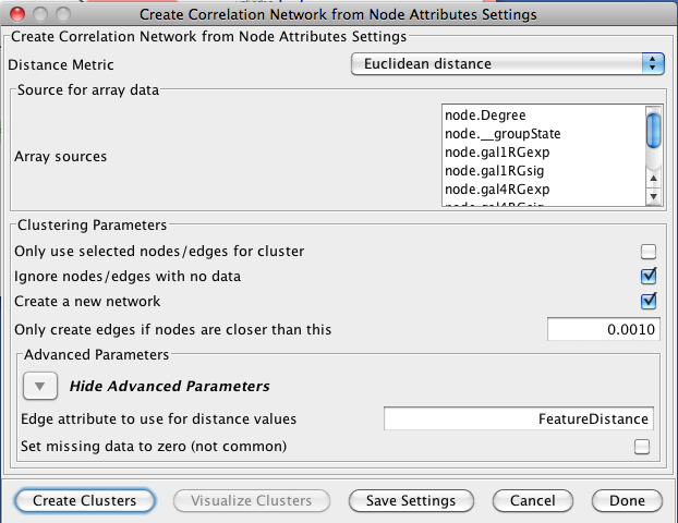
Figure 4. clusterMaker Create Correlation Network dialog.
- Distance Matrix:
- There are several ways to calculate the distance matrix that is used to
build the cluster. In clusterMaker these distances represent the
distances between two rows (usually representing nodes) in the matrix.
clusterMaker currently supports eight different metrics:
- Euclidean distance: this is the simple two-dimensional Euclidean distance between two rows calculated as the square root of the sum of the squares of the differences between the values.
- City-block distance: the sum of the absolute value of the differences between the values in the two rows.
- Pearson correlation: the Pearson product-moment coefficient of the values in the two rows being compared. This value is calculated by dividing the covariance of the two rows by the product of their standard deviations.
- Pearson correlation, absolute value: similar to the value above, but using the absolute value of the covariance of the two rows.
- Uncentered correlation: the standard Pearson correlation includes terms to center the sum of squares around zero. This metric makes no attempt to center the sum of squares.
- Uncentered correlation, absolute value: similar to the value above, but using the absolute value of the covariance of the two rows.
- Spearman's rank correlation: Spearman's rank correlation (�) is a non-parametric measure of the correlation between the two rows. This metric is useful in that it makes no assumptions about the frequency distribution of the values in the rows, but it is relatively expensive (i.e., time-consuming) to calculate.
- Kendall's tau: Kendall tau rank correlation coefficient (Ï„) between the two rows. As with Spearman's rank correlation, this metric is non-parametric and computationally much more expensive than the parametric statistics.
- None -- attributes are correlations: No distance calculations are performed. This assumes that the attributes are already correlations (probably only useful for edge attributes). Note that the attributes are also not normalized, so the correlations must be between 0 and 1.
- Array sources:
- This area contains the list of all numeric node attributes that can be used for calculating the distances between the nodes. One or more node attributes must be selected to perform the clustering.
- Only use selected nodes/edges for cluster:
- Under certain circumstances, it may be desirable to cluster only a subset of the nodes in the network. Checking this box limits all of the clustering calculations and results to the currently selected nodes or edges.
- Create a new network
- If this option is selected, then a new network will be created with all of the nodes and the edges which represent the correlation between the nodes. An edge will only be created if the nodes are closer than the value specified in the next option. If this option is not selected, an attribute will be added to existing edges with the value of the correlation.
- Only create edges if nodes are closer than this:
- This value indicates the maximum correlation to consider when determining whether to create an edge or not. The correlation values are all normalized to lie between 0 and 1.
- Advanced Parameters
- Edge attribute to use for distance values
- This is the name of the attribute to use for the distance values.
- Set missing data to zero
- In some circumstances (e.g. hierarchical clustering of edges) it is desirable to set all missing edges to zero rather than leave them as missing. This is not a common requirement.
3.3 Hierarchical Clustering
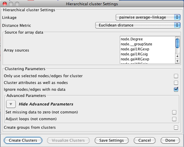
Figure 5. clusterMaker Hierarchical cluster dialog.
- Linkage:
- In agglomerative clustering techniques such as hierarchical clustering,
at each step in the algorithm, the two closest groups are chosen to be merged.
In hierarchical clustering, this is how the dendrogram (tree) is constructed.
The measure of "closeness" is called the linkage between the two groups.
Four linkage types are available:
- pairwise average-linkage: the mean distance between all pairs of elements in the two groups
- pairwise single-linkage: the smallest distance between all pairs of elements in the two groups
- pairwise maximum-linkage: the largest distance between all pairs of elements in the two groups
- pairwise centroid-linkage: the distance between the centroids of all pairs of elements in the two groups
- Distance Matrix:
- There are several ways to calculate the distance matrix that is used to
build the cluster. In clusterMaker these distances represent the
distances between two rows (usually representing nodes) in the matrix.
clusterMaker currently supports eight different metrics:
- Euclidean distance: this is the simple two-dimensional Euclidean distance between two rows calculated as the square root of the sum of the squares of the differences between the values.
- City-block distance: the sum of the absolute value of the differences between the values in the two rows.
- Pearson correlation: the Pearson product-moment coefficient of the values in the two rows being compared. This value is calculated by dividing the covariance of the two rows by the product of their standard deviations.
- Pearson correlation, absolute value: similar to the value above, but using the absolute value of the covariance of the two rows.
- Uncentered correlation: the standard Pearson correlation includes terms to center the sum of squares around zero. This metric makes no attempt to center the sum of squares.
- Uncentered correlation, absolute value: similar to the value above, but using the absolute value of the covariance of the two rows.
- Spearman's rank correlation: Spearman's rank correlation (�) is a non-parametric measure of the correlation between the two rows. This metric is useful in that it makes no assumptions about the frequency distribution of the values in the rows, but it is relatively expensive (i.e., time-consuming) to calculate.
- Kendall's tau: Kendall tau rank correlation coefficient (Ï„) between the two rows. As with Spearman's rank correlation, this metric is non-parametric and computationally much more expensive than the parametric statistics.
- None -- attributes are correlations: No distance calculations are performed. This assumes that the attributes are already correlations (probably only useful for edge attributes). Note that the attributes are also not normalized, so the correlations must be between 0 and 1.
- Array sources:
- This area contains the list of all numeric node attributes that can be used for calculating the distances between the nodes. One or more node attributes must be selected to perform the clustering.
- Only use selected nodes/edges for cluster:
- Under certain circumstances, it may be desirable to cluster only a subset of the nodes in the network. Checking this box limits all of the clustering calculations and results to the currently selected nodes or edges.
- Cluster attributes as well as nodes:
- If this box is checked, the clustering algorithm will be run twice, first with the rows in the matrix representing the nodes and the columns representing the attributes. The resulting dendrogram provides a hierarchical clustering of the nodes given the values of the attributes. In the second pass, the matrix is transposed and the rows represent the attribute values. This provides a dendrogram clustering the attributes. Both the node-based and the attribute-base dendrograms can be viewed, although Cytoscape groups are only formed for the node-based clusters.
- Ignore nodes with no data:
- A common use of clusterMaker is to map expression data onto a pathway or protein-protein interaction network. Often the expression data will not cover all of the nodes in the network, so the resulting dendrogram will have a number of "holes" that might make interpretation more difficult. If this box is checked, only nodes that have values for at least one of the attributes will be included in the matrix.
- Advanced Parameters:
- Set missing data to zero:
- In some circumstances (e.g. hierarchical clustering of edges) it is desirable to set all missing edges to zero rather than leave them as missing. This is not a common requirement.
- Adjust loops:
- In some circumstances (e.g. hierarchical clustering of edges) it's useful to set the value of the edge between and node and itself to a large value. This is not a common requirement.
- Create groups from clusters:
- If this button is checked, hierarchical Cytoscape groups will be created from the clusters. Hierarchical groups can be very useful for exploring the clustering in the context of the network. However, if you intend to perform multiple runs to try different parameters, be aware that repeatedly removing and recreating the groups can be very slow.
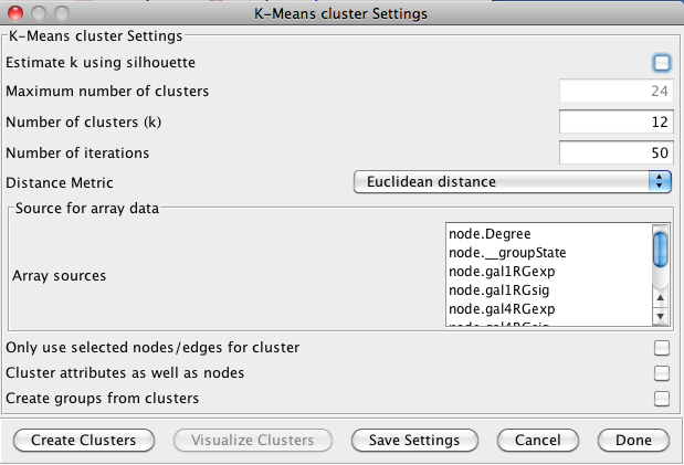
Figure 6. clusterMaker K-Means cluster dialog.
3.4 K-Means Clustering
K-Means clustering is a partitioning algorithm that divides the data into k non-overlapping clusters, where k is an input parameter. One of the challenges in k-Means clustering is that the number of clusters must be chosen in advance. A simple rule of thumb for choosing the number of clusters is to take the square root of ½ of the number of nodes. Beginning with clusterMaker version 1.6, this value is provided as the default value for the number of clusters. Beginning with clusterMaker version 1.10, k may be estimated by iterating over number of estimates for k and choosing the value that maximizes the silhouette for the cluster result. Since this is an iterative approach, for larger clusters, it can take a very long time, even though the process is multi-threaded. The K-Means cluster algorithm has several settings:- Estimate k using silhouette
- If this is checked, clusterMaker will perform k-means iteratively trying different values for k. It will then choose the value of k that maximizes the average silhouette over all clusters.
- Maximum number of clusters
- This is the maximum value for k that will be attempted when using silhouette to choose k.
- Number of clusters (k)
- This is the value clusterMaker will use for k if silhouette is not being used.
- Number of iterations
- The number of iterations in the k-means algorithm.
3.5 K-Medoid Clustering
K-Medoid clustering is essentially the same as K-Means clustering except that the medoid of the cluster is used rather than the means to determine the goodness of fit. All other options are the same.4. Network Cluster Algorithms
The primary function of the network cluster algorithms is to detect natural groupings of nodes within the network. These groups are generally defined by a numeric edge attribute that contains some similarity or distance metric between two nodes, although some algorithms function purely on the existance of an edge (i.e. the connectivity). Nodes that are more similar (or closer together) are more likely to be grouped together.
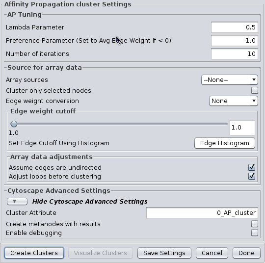
Figure 7. clusterMaker Affinity Propagation cluster dialog.
4.1 Affinity Propagation
Affinity Progation models the flow of data between points in a network in order to determine which of the points serve as data centers. These data centers are referred to as exemplars.Initally, AP considers all data points as potential exemplars. Real-valued messages are exhanged between data points at each iteration. The strength of the transmited messages determine the extent to which any given point serves as an exemplar to any other point. The quality of possible exemplar assignment is determined by a squared error energy function. Eventually, the algorithm reaches a minimal energy based on a good set of exemplars. The exemplars are then used to ouput the corresonding clusters. AP takes as input three parameters, which are discussed below.
AP Tuning
- Lambda Parameter:
- This parameter dampens the strengh of the message exchange at each iteration. Damping is necessary to avoid numerical oscillations that arise in some circumstances. Lambda may from 0 to .1. The default damping faction .5 tends to give adequate results.
- Preference Parameter:
- This parameter determines cluster density. It is analogous to the inflation parameter in MCL. Larger values for the preference parameter yield more clusters. If specified as less then zero, the preference value is automatically reset to the average edge weight in the network
- Number of iterations:
- Number of iterations the message exchange is run. 10 is usually enough to yield a stable set of exemplars
Source for array data
- Array sources:
- This pulldown contains all of the numeric edge attributes that can be used for this cluster algorithm. If is selected, all edges are assumed to have a weight of 1.0.
- Cluster only selected nodes:
- If this checkbox is selected, only the nodes (and their edges) which are selected in the current network are considered for clustering. This can be very useful to apply a second clustering to a cluster using a different algorithm or different tuning values.
- Edge weight conversion:
- There are a number of conversions that might be applied to the edge weights before clustering:
- None: Don't do any conversion
- 1/value: Use the inverse of the value. This is useful if the value is a distance (difference) rather than a similarity metric.
- LOG(value): Take the log of the value.
- -LOG(value): Take the negative log of the value. Use this if your edge attribute is an expectation value.
- SCPS: The paper describing the SCPS (Spectral Clustering of Protein Sequences) algorithm uses a special weighting for the BLAST expectation values. This edge weight conversion implements that weighting.
- Edge weight cutoff:
- Some clustering algorithms (e.g. MCL) have problems clustering very dense networks, even though many of the edge weights are very small. This value allows the user to set a custoff, either by directly entering a value, or using a slider to adjust the parameter. To view the histogram of edge weights (and set the edge weight cutoff on the histogram) use the Edge Histogram button.
- Edge Histogram button
- The edge weight histogram dialog provides an interface to allow users to explore the histogram of edge
weights and interactively set the edge weights by dragging a slider along the histogram. The dialog supports five
buttons:
- Set Cutoff This puts a vertical line on the graph and allows the user to drag the line along to set the cutoff value. You must click into the historgram after pressing the button to activate the verticle line. The value and number of edges with that value are displayed at the top of the line (See Figure 8). The slider sets the value as it is dragged, so no further action is necessary once the desired cutoff is selected.
- Close Close the dialog.
- Zoom In Zooms in to the dialog (multiplies the width by 2). The histogram is placed in a scroll window so that the user may continue to have access to the entire histogram. This button may be pressed repeatedly.
- Zoom Out If the user has expanded the dialog with the Zoom In button, this button allows the user to zoom back out.
- Select Cutoff Heuristically This will calculate a candidate cutoff using the heuristic proposed by Apeltsin, et. al. (2011).
- Assume edges are undirected:
- Some clustering algorithms take the edge direction into account, althrough most do not. Assuming the edges are undirected is normal. Not all algorithms support this value.
- Adjust loops before clustering:
- Loops refere to edges between a node and itself. Most networks do not include these as they cluster the visualization and don't seem informative. However, mathematically when the network is converted to a matrix these values become important. Checking this box sets these self-edges to the largest value of any edge in the row. Not all algorithms support this value.
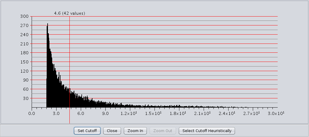
Figure 8. clusterMaker Edge Weight Histogram dialog with the Set Cutoff slider enabled.
Cytoscape Advanced Settings
- Cluster Attribute:
- Set the node attribute used to record the cluster number for this node. Changing this values allows multiple clustering runs using the same algorithm to record multiple clustering assignments.
- Create metanodes with results:
- Selecting this value directs the algorithm to create a Cytoscape metanode for each cluster. This allows the user to collapse and expand the clusters within the context of the network.
- Enable debugging:
- Some algorithms have debugging statements that will display via the Cytoscape logger. Selecting this will enable them, but you may still need to select the corresponding property in Cytoscape to enable display of the debug log.
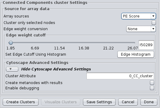
Figure 9. clusterMaker Connected Components cluster dialog.
4.2 Connected Components
This is a very simple "cluster" that simply finds all of the disconnected components of the network and treats each disconnected component as a cluster. It supports the Array Sources and the Cytoscape Advanced Settings options. Figure 9 shows the options panel for the Connected Components cluster, which essentially has only the Array Sources and Cytoscape Advanced Settings options.
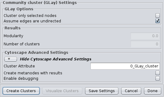
Figure 10. clusterMaker Community cluster (GLay) dialog.
4.3 Community Clustering (GLay)
The community clustering algorithm is an implementation of the Girvan-Newman fast greedy algorithm as implemented by the GLay Cytoscape plugin. This algorithm operates exclusively on connectivity, so there are no options to select an array source, although options are provided to Cluster only selected nodes and Assume edges are undirected. It supports all of the Cytoscape Advanced Settings options.
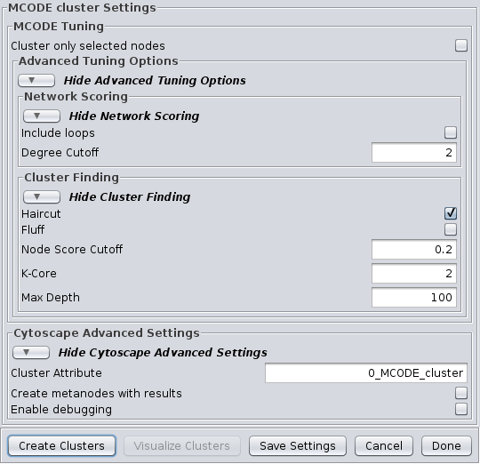
Figure 11. clusterMaker MCODE cluster dialog.
4.4 MCODE
The MCODE algorithm finds highly interconnected regions in a network. The algorithm uses a three-stage process:
- Vertex weighting, which weights all of the nodes based on their local network density.
- Molecular complex prediction, staring with the highest-weighted node, recursively move out adding nodes to the complex that are above a given threshold.
- Post-processing, which applies filters to improve the cluster quality.
Advanced Tuning Options
Network Scoring
- Include loops:
- If checked, loops (self-edges) are included in the calculation for the vertex weighting. This shouldn't have much impact
- Degree Cutoff:
- This value controls the minimum degree necessary for a node to be scored. Nodes with less than this number of connections will be excluded.
Cluster Finding
- Haircut:
- If checked, drops all of nodes from a cluster if they only have a single connection to the cluster.
- Fluff:
- If checked, after haircutting (if checked) all of the cluster cores are expanded by one step and added to the cluster if the score is greater than the Node Score Cutoff.
- K-Core:
- Filters out clusters that do not conatin a maximally interconnected sub-cluster of at least k degrees.
- Max Depth:
- This controls how far out from the seed node the algorithm will search in the molecular complex prediction step.
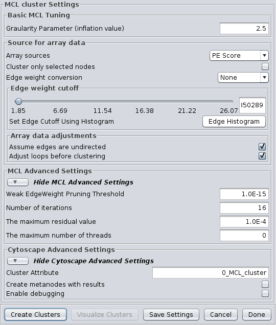
Figure 12. clusterMaker MCL cluster dialog.
4.5 MCL
Markov CLustering Algorithm (MCL) is a fast divisive clustering algorithm for graphs based on simulation of the flow in the graph. MCL has been applied to complex biological networks such as protein-protein similarity networks. As with all of the clustering algorithms, the first step is to create a matrix of the values to be clustered. For MCL, these values must be stored in edge attributes. Once the matrix is created, the MCL algorithm is applied for some number of iterations. There are two basic steps in each iteration of MCL. First is the expansion phase where the matrix is expanded by calculating the linear algebraic matrix-matrix multiplication of the original matrix times an empty matrix of the same size. The next step is the inflation phase where the each non-zero value in the matrix is raised to a power followed by performing a diagonal scaling of the result. Any values below a certain threshold are dropped from the matrix after the normalization (scaling) step in each iteration. This process models the spreading out of flow during expansion, allowing it to become more homogeneous, then contracting the flow during inflation, where it becomes thicker in regions of higher current and thinner in regions of lower current. This version of the MCL algorithm has been parallelized to improve performance on multicore processors.
The MCL dialog is shown in Figure 12. MCL has one parameter and supports the Array Sources and the Cytoscape Advanced Settings options, as well as a set of four advanced settings. Each parameter is discussed below:
- Granularity Parameter (inflation value)
- The Granularity Parameter is also known as the inflation parameter or inflation value. This is the power used to inflate the matrix. Reasonable values range from ~1.8 to about 2.5. A good starting point for most networks is 2.0.
MCL Advanced Settings
- Weak Edge Weight Pruning Threshold
- After each inflation pass, very small edge weights are dropped out. This should be a very small number: 1x10⁻¹⁰ or so. The algorithm is more sensitive to tuning this parameter than it is to tuning the inflation parameter. Changes in this parameter also significantly impact the performance.
- Number of iterations
- This is the maximum number of iterations to execute the algorithm.
- The maximum residual value
- After each iteration, the residuals are calculated, and if they are less than this value, the algorithm is terminated. Set this value very small to ensure that you get sufficient iterations.
- The maximum number of threads
- If the machine has multiple cores or CPUs, MCL will by default utilize nCPUs-1 for it's operations. So, on an Intel i7 with 4 cores and hyperthreading, MCL will utilize 7 threads (4 cores X 2 hyperthreads) - 1 = 7. If this parameter is set to something other than 0, MCL will ignore the above calculation and utilize the specified number of threads.
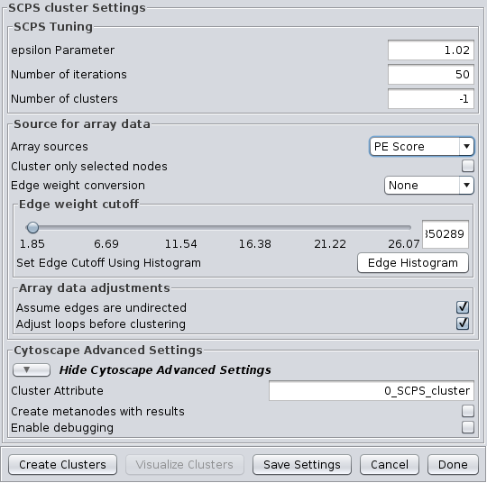
Figure 13. clusterMaker SCPS cluster dialog.
4.6 SCPS (Spectral Clustering of Protein Sequences)
SCPS is a spectral method designed for grouping proteins. Spectral methods use the eigenvalues in an input similarity matrix to perform dimensionality reduction for clustering in fewer dimensions. SCPS builds a matrix from the k largest eigenvectors, where k is the number of clusters to be determined. A normalized transpose of that matrix is then used as input into a standard k-means clustering algorithm. The user may specify the Number of clusters parameter with a preset value of k, as well as the Number of iterations that k-means is to be run. However, if the user does not know the value of k in advance, he or she may set the Number of clusters to -1, and SCPS will pick a value for k using an automated heuristic. The heuristic picks the smallest integer k such that the ratio of the kth eignevalue and the k+1st eigenvalue is greater then the Epsilon Paramter. An epsilon of 1.02 is good for clustering diverse proteins into superfamilies. A more granular epsilon of 1.1 may cluster proteins into functional families. SCPS supports the Array Sources and the Cytoscape Advanced Settings options.
SCPS Tuning
- epsilon Parameter:
- The epsilon parameter to use.
- Number of Iterations:
- The number of iterations for the k-means clustering.
- Number of clusters:
- The number of clusters. If this is -1, SCPS will pick a value for k using an automated heuristic.
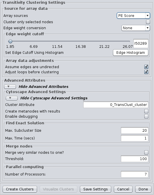
Figure 14. clusterMaker Transitivity cluster dialog.
4.7 Transitivity Clustering
TransClust is a clustering tool that incorporates the hidden transitive nature occuring within biomedical datasets. It is based on weighed transitive graph projection. A cost function for adding and removing edges is used to transform a network into a transitive graph with minimal costs for edge additions and removals. The final transitive graph is by definition composed of distinct cliques, which are equivalent to the clustering output. Transitivity Clustering supports the Array Sources and the Cytoscape Advanced Settings options.
Advanced Attributes
Find Exact Solution
- Max. Subcluster Size:
- The maximum size of a subcluster. This option adjusts the size of subproblems to be saved exactly. The higher the number, the higher the running time but also the accuracy. For fast computers, you may want to set this value to 50.
- Max. Time (secs):
- The maximum time, in seconds, to execute each loop in the algorithm. Increasing this parameter raises both running time and accuracy. For fast computers, you may want to set this value to 2.
Merge nodes
- Merge very similar nodes to one?:
- If this it true, nodes exceeding a threshold parameter will be merged be merged virtually into one object while clustering. This may decrease running time drastically.
- Threshold:
- The threshold for merging nodes the merge parameter is activated. For protein sequence clustering using BLAST as a smiliarity function, it might make sense to set the threshold at 323, since this is the highest reachable similarity.
Parallel computing
- Number of Processors:
- The number of processors (threads) to use.
5. Filtering Clusters
Filters are a tool to "fine tune" clusters after a clustering algorithm has completed. In general, the idea behing the filters are to examine the results of a clustering algorithm and, based on some metric, trim the edges (drop nodes) or add edges to improve the clustering. The goal is to reduce noise and increase the cluster quality.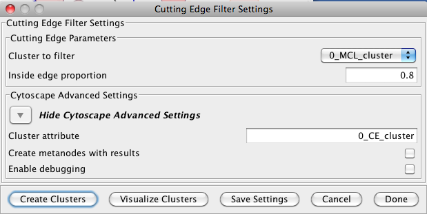
Figure 15. The settings dialog for the Cutting Edge Filter.
5.1 Cutting Edge Filter
Cutting Edge is a relatively coarse filter that discards clusters that don't meet the criteria. The criteria is defined as a density value where the cluster density is equal to the number of intra-cluster edges divided by the total number of edges (both intra-cluster and inter-cluster) that connect to nodes belonging to this cluster. If the density is less than the value, the cluster is dropped. The Cutting Edge Filter has the following values:- Cluster to filter
- This is the attribute that contains the cluster numbers to use for the filtering.
- Inside edge proportion
- The proportion of inside edges to total edges. Values can vary from 0 to 1 where 0 implies that the cluster has no inside edges and 1 implies that all of the edges are inside edges.
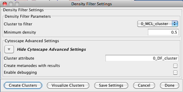
Figure 16. The settings dialog for the Density Filter.
5.2 Density Filter
This filter drops clusters which have an edge density beneath the user-defined threshold. A fully connected network (all nodes are connected to all other nodes) will have an edge density of 1. A completely disconnected network will have an edge density of 0. The Density Filter has the following values:- Cluster to filter
- This is the attribute that contains the cluster numbers to use for the filtering.
- Minimum density
- The minimum density a cluster must have to be retained, where 0 implies that the cluster has no inside edges and 1 implies that all of the nodes are connected to all other nodes (fully connected).
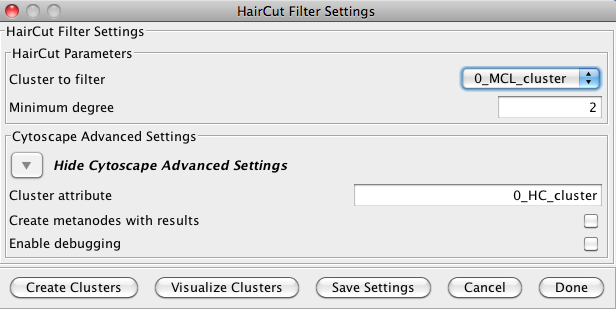
Figure 17. The settings dialog for the Haircut Filter.
5.3 Haircut Filter
The haircut filter removes nodes from a cluster that have a degree (number of incident edges) below a specified value. The idea is that the lower the connectivity of a node, the lower the probability for this node to really belong to the cluster it is in. The Haircut Filter has the following values:- Cluster to filter
- This is the attribute that contains the cluster numbers to use for the filtering.
- Minimum degree
- This is the minimum degree for a node to be kept within the cluster.
6. Visualizing Results
clusterMaker provides two basic approaches for visualizations: Heat Maps and Networks. clusterMaker provides three options for network display: Create New Network from Attribute, Create New Network from Clusters, and Create New Network with Nested Networks from Attribute; and three types of heat map display: HeatMapView (unclustered), Eisen TreeView, and Eisen KnnView.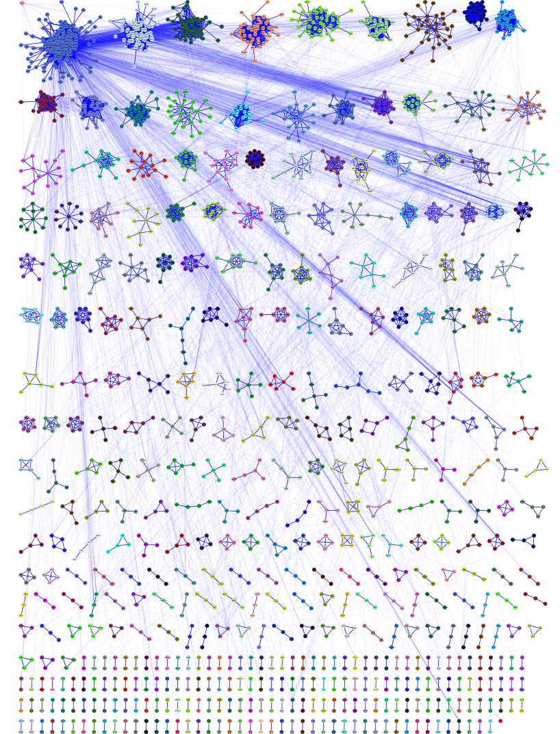
Figure 18. The network created by clusterMaker's MCL clustering algorithm for MS/TAP protein-protein interaction data from yeast. The network was created by using Create New Network from Attribute and selecting the option to add inter-cluster edges back.
6.1 Create New Network from Attribute
This menu item can be used to create a network from any numerical attribute, where only the nodes with the same values of the attribute are connected. Note that there is no binning of these values, so using continues values would result in clusters that make little sense. There are two options on the dialog:
- Display only selected nodes (or edges)
- Self-explanatory, the new network will contain only the nodes selected in the current network
- Restore inter-cluster edges after layout
- If this option is selected, the resulting network will be created with only the intra-cluster edges. Then, after the network is laid out (and partitioned as a result) the inter-cluster edges will be added back in.
6.2 Create New Network from Clusters
This menu item will be selectable if a network cluster algorithm has completed and stored the cluster numbers in a node attribute. When selected, this menu will create a new network that contains only the intra-cluster edges, then layout that network using the unweighted force-directed layout algorithm. All inter-cluster edges will be dropped. If there is value in visualizing the network with the inter-cluster edges also, see the Create New Network from Attribute menu item above.
6.3 Create New Network with nested networks from attribute
This does pretty much the same as the Create New Network from Attribute except that each cluster is created as a separate network, then a single network is created where each cluster network is represented as a nested network. WARNING: this can be memory and performance intensive if there are a large number of clusters This dialog has only one option:
- Display only selected nodes (or edges)
- Self-explanatory, the new network will contain only the nodes selected in the current network
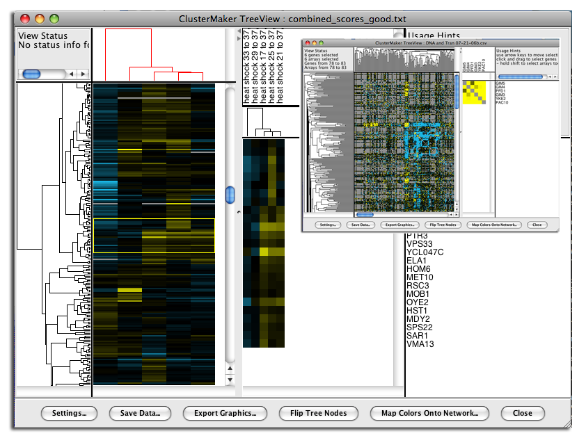
Figure 19. clusterMaker's Eisen TreeView. The larger image shows the results of hierarchically clustering the nodes and five node attributes (expression data from a heat shock experiment). The inset shows the results of hierarchical clustering using an edge attribute. The resulting network is symmetrical across the diagonal, and the dendrograms at the left and top are the same.
6.4 Eisen TreeView
Hierarchical clustering results are usually displayed with the Eisen TreeView (see Figure 19). This view provides a color-coded "Heat Map" of the data values and the dendrogram from clustering. The Eisen TreeView can be created by clicking on the Visualize Clusters button in the Hierarchical cluster dialog (Figure 4) or by selecting Plugin→Cluster→Eisen TreeView from the Cytoscape tool bar. Note that both of these methods will be "grayed out" unless hierarchical clustering has been performed on the current network. The information necessary to create the TreeView is retained across sessions (stored in network attributes), so these options should be available when you reload a session that had been saved after hierarchical clustering.The basic TreeView window has four main vertical windows: Node Dendrogram, Global HeatMap, Zoom HeatMap, and the Node List. These windows may be resized to emphasize different portions of the TreeView. Each of the windows is discussed in detail below. Note that selection of a row in TreeView will select the corresponding node in the current network view in Cytoscape (if that node exists). The reverse is also true -- selection in Cytoscape will select the corresponding nodes in TreeView. This is an important feature of clusterMaker: multiple views (current network, multiple heat maps if present) respond simultaneously to a selection in any one view.
- Node Dendrogram
- The leftmost pane displays the node dendrogram for the heat map. At the top of the pane is a
Status window that changes depending on the
location of the pointer. With the pointer over the
node dendrogram, the Status window will display
the ID and correlation for the currently selected
branch of the dendrogram (if any). If the cursor is over the
Global HeatMap window the Status window
displays the number of genes (nodes) and arrays (attributes) selected and the range of the selections.
Finally, if the cursor is over the Zoom HeatMap window, the
Status window displays the node and attribute name as well as
the value of the spot under the pointer.
Mouse and keyboard actions in node dendrogram pane Action Target Result click Dendrogram branch Select that branch of the dendrogram and all children up arrow  If there is a currently selected branch, select its parent and all subsequent children down arrow  If there is a currently selected branch, move to the top branch and deselect the bottom branch left arrow  If there is a currently selected branch, move to the top branch and deselect the bottom branch right arrow  If there is a currently selected branch, move to the bottom branch and deselect the top branch - Global HeatMap
- The Global HeatMap is the next pane over,
divided into
two parts. The upper part contains the dendrogram for the attributes (if they were clustered) and the
lower part contains the entire heat map in a scrolling window.
Horizontal and vertical scroll bars will be provided as needed.
Selection of branches in the dendrogram in the upper window
is similar to that in the node dendrogram (see above). Selections in the
Global HeatMap pane
are shown with a thin yellow outline. The area corresponding to the
Zoom HeatMap view is shown with
a thin blue outline.
Mouse and keyboard actions in global heatmap pane Action Target Result + Heat map Zoom the global view by 2X - Heat map Zoom the global view by 1/2 (but not smaller than 1 pixel in width or height for each cell) click Heat map Select that row of the heat map shift-click Heat map Select that cell of the heat map drag Heat map Select the rows encompassed by the dragged-out region shift-drag Heat map Select the region encompassed by the dragged-out area up arrow  If there is a current selection, move that selection up one row down arrow  If there is a current selection, move that selection down one row left arrow  If there is a current selection, move that selection left one column right arrow  If there is a current selection, move that selection right one column control-up arrow  If there is a current selection, expand that selection by two rows (one on the top and one on the bottom) control-down arrow  If there is a current selection, contract that selection by two rows (one on the top and one on the bottom) control-left arrow  If there is a current selection, expand that selection by two columns (one on the left and one on the right) control-right arrow  If there is a current selection, contract that selection by two columns (one on the left and one on the right) - Zoom HeatMap
- The Zoom HeatMap view shows the nodes and attributes selected in the Global HeatMap window. It has three sections: the top section lists the names of the attributes that correspond to the columns in the heat map, the next section down contains the dendrogram for the columns (if one was calculated), and the bottom section contains the heat map itself. There are no mouse or keyboard actions in the top or bottom windows, but if a dendrogram is present, it will respond to mouse and keyboard actions in the same way as the Global HeatMap dendrogram.
- Node List
- Finally, the right-most pane lists each node shown in the Zoom HeatMap pane. The list is sized to correspond exactly to the rows in the Zoom HeatMap pane and scrolls along with it so that the names stay aligned with the rows.
- Settings...
- Save Data...
- Export Graphics...
- Flip Tree Nodes (in the Eisen TreeView dialog only)
- Map Colors Onto Network...
- Close
Figure 20. Pixel Settings Dialog.
- Settings...
- The Settings... button brings up the Pixel Settings dialog, which allows
users to customize the dimensions of heat map cells in the
Global and Zoom panes.
The dimensions can be specified as pixel values
(Fixed scale) for
X (width) and Y (height),
or to automatically fill the available space (Fill).
Users can specify which color scheme should be used: a red-green (RedGreen) continuum or the default yellow-blue (YellowBlue). Color schemes may also be customized by setting the Positive, Zero, Negative, and Missing values. Once these values have been assigned, they can be saved as presets (Make Preset). The Load... and Save.. buttons are used to load and save color sets, respectively.
The Pixel Settings dialog also provides a Contrast slider to adjust the contrast of the colors. This is useful to emphasize more subtle differences in heat map values. Finally, LogScale rather than a linear mapping of values to colors can be used, and the center point set to improve the display of single-tailed data.
- Save Data...
- In order to facilitate data exchange and analysis by other software, the Save Data... button will export the current data in Cluster format, including the .cdt, .gtr, and .atr files, as appropriate.
- Export Graphics...
-
The Export Graphics... button brings up the Export Graphics Dialog (see
Figure 21), which
provides an interface to export the heat map to a variety of different graphics formats:
Graphics Formats Supported by clusterMaker Format Type Quality png Bitmap highest bitmap quality jpg Bitmap reasonable bitmap quality, but aberrations visible at high scales bmp Bitmap very good bitmap quality pdf Vector excellent quality svg Vector excellent quality, but not widely supported eps Vector excellent quality, but will need to be processed by a separate program 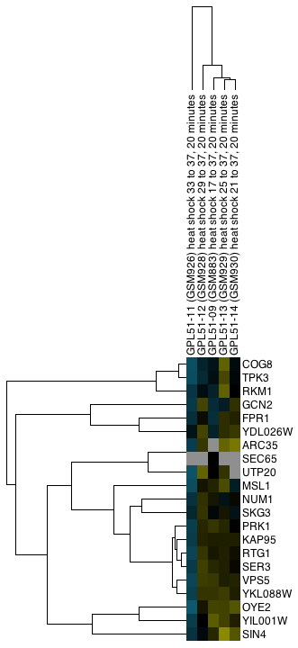
Figure 22. Example export of a portion of a TreeView heat map showing both the Node and Attribute dendrograms (click on the image to see a larger version).
Generally, vector formats yield a higher-quality appearance, as they can be scaled. Particularly for use in a graphics package such as Adobe Illustrator or Adobe Photoshop, vector formats are much preferred. For inclusion in a web page or presentation, png is a reasonable choice if you are not planning on doing any significant zooming and cropping (see Figure 22).
Options for what is included in the output depend on the type of display. For TreeView heat maps that are symmetric (i.e., created using an edge attribute), the Left Node Tree and the Top Node Tree may be included in the output, and you will almost always want to include the Heat Map itself. For TreeView heat maps with both nodes and attributes clustered, you will be able to include the Node Tree, Attribute Tree, and the Heat Map. If the attributes were not clustered, the Attribute Tree will not be available.
If only part of the heat map is desired, you can choose to save just the selected portion (Selection Only). Note that to include dendrograms in the output, you will need to select a full subtree.
- Flip Tree Nodes
- The Flip Tree Nodes button will flip the order of the trees in the top dendrogram, if it exists. At this time, there is no corresponding way to flip the left dendrogram.
- Map Colors Onto Network...
-
The Map Colors Onto Network... button provides a method for mapping the
colors from the heat map back onto Cytoscape nodes (and edges for symmetric heat maps). If a
single column (attribute) is selected, a new VizMap will be created and the colors corresponding to that
attribute will be assigned to the nodes in the network view. If multiple columns are selected, the
Map Colors to Network
dialog (shown in Figure 23 below) will be displayed. From this dialog, you will be able to
select a single attribute and create the VizMap for that attribute, or select multiple attributes to
create a VizMap for each attribute and animate through them. An Animation Speed
slider allows the user to select the speed of the animation. The initial pass will take slightly
longer as the VizMap for each attribute needs to be created, but after that, the animation speed
should correspond closely to the slider. If the nodeCharts plugin is loaded, you will also
be able to create "HeatStrips", which are small bar-charts that represent the heat map values, that
will appear under the corresponding nodes in the network view.
NOTE: At this time, there is no way to save the animation as a movie, although this is a much-requested feature and will be implemented in the future.
- Close
- The Close button closes the dialog.
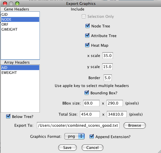
Figure 21. Export Graphics Dialog.
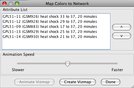
Figure 23. The Map Colors to Network Dialog
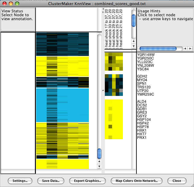
Figure 24. The Eisen KnnView dialog showing the results of visualizing a k-Means cluster with k=30.
6.5 Eisen KnnView
The results of k-Means clustering can be shown with the Eisen KnnView (Figure 24). This is much the same as the Eisen TreeView discussed above, except that the dendrogram areas are empty and the clusters are separated by a blank space the width of one cell. All of the features discussed as part of the Eisen TreeView are available in the Eisen KnnView except the Flip Tree Nodes button, and the Node Tree and Attribute Tree options are not available in the Export Graphics dialog.6.6 HeatMapView (unclustered)
Any attribute or group of attributes may be shown as a heat map using the clusterMaker HeatMapView (unclustered). The dialog is identical to the Eisen KnnView except that since there are no clusters, there are no blank spaces separating the clusters.7. Interaction
7.1 Link network selection
This menu links selection between all of the current Cytoscape networks. If a node is selected in one network, and that node exists in any other network, it will be selected in that network also. This is useful for comparing clustering results, or any other network comparison.
8. Commands
The clusterMaker plugin registers two different namespaces (top-level commands) that are available to scripts or to other plugins: clustermaker and clusterviz. Each of these is discussed in turn below.
8.1 clustermaker command
The clustermaker commmand provides an interface to the clustering algorithms. Each algorithm is a sub-command. In addition to the algorithm commands, there is a command to show the clusterMaker dialog for an algorithms, a command to check to see if a cluster has already been performed on a network, a command to return the results of an attribute cluster algorithm, and a command to return the results of a network cluster algorithm. The non-algorithm commands will be listed first, followed by the commands for each algorithm.
- clustermaker hascluster
-
See if a cluster algorithm has been run on a network.
Arguments:
- type=algorithm: The algorithm to check for results for
- clustermaker getcluster
-
Retreive previously calculated attribute clusters.
Arguments:
- clustertype=[node|attribute]: Whether to return the clusters for nodes or attributes.
- type=[hierarchical|kmeans|kmedoid|autosome]: The algorithm to get results for
- clustermaker getnetworkcluster
-
Retreive previously calculated network clusters.
Arguments:
- type=algorithm: The algorithm to get results for
- clustermaker ap
-
Partition the network using Affinity Propagation.
Arguments:
- lambda=0.5: Lambda Parameter.
- preference=-1: Preference Parameter (Set to Avg Edge Weight if < 0).
- iterations=10: Number of iterations
- attribute=attribute: Array sources
- selectedOnly=false: Cluster only selected nodes
- edgeWeighter=[--None--|1/value|-LOG(value)|LOG(value)|SCPS]: Edge weight conversion
- edgeCutOff=cutoff: Edge weight cutoff
- undirectedEdges=[true|false]: Assume edges are undirected
- adjustLoops=[true|false]: Adjust loops
- clusterAttrName=attributeName: Cluster Attribute
- createGroups=false: Create metanodes with results
- debug=false: Enable debugging
- clustermaker autosome_heatmap
-
Cluster using AutoSOME assuming attribute-based clustering.
Arguments:
- mode=[Normal|Precision|Speed]: Running Mode
- ensembleRuns=50: Number of Ensemble Runs
- pvalueThresh=0.05: P-Value Threshold
- numThreads=threads: Number of Threads (No. CPUs)
- norm_mode=[Custom|No normalization| Expression data 1|Expression data 2]: Normalization mode
- logScaling=false: Log2 Scaling
- unitVariance=false: Unit Variance
- medCenter=[None|Genes|Arrays|Both]: Median Centering
- sumSquares=[None|Genes|Arrays|Both]: Sum of Squares=1
- enableFCN=false: Perform Fuzzy Clustering
- FCNInput=[Nodes (Genes)|Attributes (Arrays)]: Source Data
- FCNmetric=[Uncentered Correlation|Pearson's Correlation|Euclidean]: Distance Metric
- maxEdges=2000: Maximum number of edges to display in fuzzy network
- attributeList=cluster attributes: Array Sources (Node Attributes)
- selectedOnly=false: Cluster only selected nodes
- ignoreMissing=true: Ignore nodes/edges with no data
- cluster_output=Heatmap: Choose Visualization
- clustermaker autosome_network
-
Cluster using AutoSOME assuming network-based clustering.
Arguments:
- mode=[Normal|Precision|Speed]: Running Mode
- ensembleRuns=50: Number of Ensemble Runs
- pvalueThresh=0.05: P-Value Threshold
- numThreads=threads: Number of Threads (No. CPUs)
- norm_mode=[Custom|No normalization| Expression data 1|Expression data 2]: Normalization mode
- logScaling=false: Log2 Scaling
- unitVariance=false: Unit Variance
- medCenter=[None|Genes|Arrays|Both]: Median Centering
- sumSquares=[None|Genes|Arrays|Both]: Sum of Squares=1
- enableFCN=false: Perform Fuzzy Clustering
- FCNInput=[Nodes (Genes)|Attributes (Arrays)]: Source Data
- FCNmetric=[Uncentered Correlation|Pearson's Correlation|Euclidean]: Distance Metric
- maxEdges=2000: Maximum number of edges to display in fuzzy network
- attributeList=cluster attributes: Array Sources (Node Attributes)
- selectedOnly=false: Cluster only selected nodes
- ignoreMissing=true: Ignore nodes/edges with no data
- cluster_output=Network: Choose Visualization
- clustermaker connectedcomponents
-
Create a cluster attribute from the connected components.
Arguments:
- attribute=attribute: Array sources
- selectedOnly=false: Cluster only selected nodes
- edgeWeighter=[--None--|1/value|-LOG(value)|LOG(value)|SCPS]: Edge weight conversion
- edgeCutOff=cutoff: Edge weight cutoff
- undirectedEdges=[true|false]: Assume edges are undirected
- adjustLoops=[true|false]: Adjust loops
- clusterAttrName=attributeName: Cluster Attribute
- createGroups=false: Create metanodes with results
- debug=false: Enable debugging
- clustermaker glay
-
Partition the network using Community Clustering (GLay).
Arguments:
- selectedOnly=false: Cluster only selected nodes
- undirectedEdges=[true|false]: Assume edges are undirected
- clusterAttrName=attributeName: Cluster Attribute
- createGroups=false: Create metanodes with results
- debug=false: Enable debugging
- clustermaker hierarchical
-
Perform a hierarchical cluster on a set of attributes or a single edge attribute.
Arguments:
- linkage=[pairwise single-linkage| pairwise maximum-linkage| pairwise average-linkage| pairwise centroid-linkage]: Linkage
- dMetric=[None -- attributes are correlations| Uncentered correlation| Pearson correlation| Uncentered correlation, absolute value| Pearson correlation, absolute value| Spearman's rank correlation| Kendall's tau| Euclidean distance| City-block distance]: Distance Metric
- attributeList=attribute: Array sources
- selectedOnly=false: Cluster only selected nodes
- clusterAtributes=false: Cluster attributes as well as nodes
- ignoreMissing=true: Ignore nodes/edges with no data
- adjustDiagonals=false: Adjust loops (not common)
- zeroMissing=false: Set missing data to zero (not common)
- createGroups=true: Create groups from clusters
- clustermaker kmeans
-
Perform a k-means cluster on a set of attributes or a single edge attribute.
Arguments:
- knumber=10: Number of clusters
- iterations=10: Number of iterations
- dMetric=[None -- attributes are correlations| Uncentered correlation| Pearson correlation| Uncentered correlation, absolute value| Pearson correlation, absolute value| Spearman's rank correlation| Kendall's tau| Euclidean distance| City-block distance]: Distance Metric
- attributeList=attribute: Array sources
- selectedOnly=false: Cluster only selected nodes
- clusterAtributes=false: Cluster attributes as well as nodes
- ignoreMissing=true: Ignore nodes/edges with no data
- createGroups=true: Create groups from clusters
- clustermaker kmedoid
-
Perform a k-medoid cluster on a set of attributes or a single edge attribute.
Arguments:
- knumber=10: Number of clusters
- iterations=10: Number of iterations
- dMetric=[None -- attributes are correlations| Uncentered correlation| Pearson correlation| Uncentered correlation, absolute value| Pearson correlation, absolute value| Spearman's rank correlation| Kendall's tau| Euclidean distance| City-block distance]: Distance Metric
- attributeList=attribute: Array sources
- selectedOnly=false: Cluster only selected nodes
- clusterAtributes=false: Cluster attributes as well as nodes
- ignoreMissing=true: Ignore nodes/edges with no data
- createGroups=true: Create groups from clusters
- clustermaker mcl
-
Partition the network using MCL.
Arguments:
- inflation_parameter=2.0: Granularity Parameter (inflation value)
- attribute=attribute: Array sources
- selectedOnly=false: Cluster only selected nodes
- edgeWeighter=[--None--|1/value|-LOG(value)|LOG(value)|SCPS]: Edge weight conversion
- edgeCutOff=cutoff: Edge weight cutoff
- undirectedEdges=[true|false]: Assume edges are undirected
- adjustLoops=[true|false]: Adjust loops
- clusteringThresh=1X10-15: Weak EdgeWeight Pruning Threshold
- iterations=16: Number of iterations
- maxResidual=.0001: The maximum residual value
- maxThreads=0: The maximum number of threads
- clusterAttrName=attributeName: Cluster Attribute
- createGroups=false: Create metanodes with results
- debug=false: Enable debugging
- clustermaker mcode
-
Partition the network using MCODE.
Arguments:
- selectedOnly=false: Cluster only selected nodes
- includeLoops=false: Include loops
- degreeCutoff=2: Degree Cutoff
- haircut=true: Haircut
- fluff=false: Fluff
- scoreCutoff=0.2: Node Score Cutoff
- kCore=2: K-Core
- maxDepth=100: Max Depth
- clusterAttrName=attributeName: Cluster Attribute
- createGroups=false: Create metanodes with results
- debug=false: Enable debugging
- clustermaker scps
-
Partition the network using SCPS.
Arguments:
- epsilon=1.02: epsilon Parameter
- iterations=50: Number of iterations
- knumber=-1: Number of clusters
- attribute=attribute: Array sources
- selectedOnly=false: Cluster only selected nodes
- edgeWeighter=[--None--|1/value|-LOG(value)|LOG(value)|SCPS]: Edge weight conversion
- edgeCutOff=cutoff: Edge weight cutoff
- undirectedEdges=[true|false]: Assume edges are undirected
- adjustLoops=[true|false]: Adjust loops
- clusterAttrName=attributeName: Cluster Attribute
- createGroups=false: Create metanodes with results
- debug=false: Enable debugging
- clustermaker showdialog
-
Show the clusterMaker dialog for the algorithms specified by 'type'.
Arguments:
- type=algorithm: The algorithm to show the dialog for
- clustermaker transclust
-
Partition the network using Transitivity Clustering.
Arguments:
- attribute=attribute: Array sources
- selectedOnly=false: Cluster only selected nodes
- edgeWeighter=[--None--|1/value|-LOG(value)|LOG(value)|SCPS]: Edge weight conversion
- edgeCutOff=cutoff: Edge weight cutoff
- undirectedEdges=[true|false]: Assume edges are undirected
- adjustLoops=[true|false]: Adjust loops
- clusterAttrName=attributeName: Cluster Attribute
- createGroups=false: Create metanodes with results
- debug=false: Enable debugging
- maxSubclusterSize=20: Max. Subcluster Size
- maxTime=1: Max. Time (secs)
- mergeSimilar=false: Merge very similar nodes to one?
- mergeThreshold=100: Threashold
- numberOfThreads=threads: Number of Processors
8.2 clusterviz command
- clusterviz heatmapview
- Create a heatmap visualization from a set of attributes
Arguments:
- attributeList=cluster attributes: the list of attributes to use for the columns of the heatmap.
- selectedOnly=[false]: Only use selected nodes (and their edges) to participate in the new network.
- clusterviz knnview
- Create a Knn-View visualization from the last K-Means clustering done
- clusterviz nestednetworkview
-
Create a nested network from a cluster or an attribute.
Arguments:
- attribute=cluster attribute: This is the attribute to use for the cluster attribute. If this isn't provided, the last network partitioning cluster attribute is used.
- selectedOnly=[false]: Only use selected nodes (and their edges) to participate in the new network.
- clusterviz newnetworkview
-
Create a new network from a cluster or an attribute.
Arguments:
- attribute=cluster attribute: This is the attribute to use for the cluster attribute. If this isn't provided, the last network partitioning cluster attribute is used.
- restoreEdges=[false]: Restore the inter-cluster edges after creating the network.
- selectedOnly=[false]: Only use selected nodes (and their edges) to participate in the new network.
- clusterviz treeview
- Create a Tree-View visualization from the last Hierarchical or AutoSOME clustering done
8. Acknowledgements
The Hierarchical and k-Means implementations of clusterMaker are based on the Cluster 3.0 C implementation (from Michiel de Hoon while at the Laboratory of DNA Information Analysis at the University of Tokyo), which was based on the original Cluster program written by Michael Eisen. The heatmap/dendrogram visualization is based on Java TreeView implemented by Alok Saldanha while at Stanford University. The MCL cluster algorithm was written based on the original thesis by Stejn van Dongen, with reference to the Java implementation by Gregor Heinrichi (see http://www.arbylon.net/projects/knowceans-mcl/doc/).
9. References
- M. B. Eisen, P. T. Spellman, P. O. Brown, and David Botstein: Cluster analysis and display of genome-wide expression patterns. PNAS, 95(25):14863-8 (1998) [PMID:9843981]
- A. J. Saldanha: Java Treeview--extensible visualization of microarray data. Bioinformatics, 20(17):3246-8 (2004). [PMID:15180930]
- M. J. L. de Hoon, S. Imoto, J. Nolan, and S. Miyano: Open Source Clustering Software. Bioinformatics, 20 (9):1453-1454 (2004). [PMID:14871861]
- A.M. Newman, J.B. Cooper: AutoSOME: a clustering method for identifying gene expression modules without prior knowledge of cluster number. BMC Bioinformatics 11:117 (2010). [PMID:20202218]
- L. Apeltsin, J.H. Morris, P.C. Babbitt, T.E. Ferrin: Improving the quality of protein similarity network clustering algorithms using the network edge weight distribution. Bioinformatics 27(3):326-333 (2011). [PMID:21118823]
- B.J. Frey, D. Dueck: Clustering by passing messages between data points. Science 315(5814):972-976 (2007). [PMID:17218491]
- M.E. Newman, M. Girvan: Finding and evaluating community structure in networks. Phys Rev E Stat Nonlin Soft Matter Phys 69(2 Pt 2):026113 (2004).
- G. Su, A. Kuchinsky, J.H. Morris, D.J. States, F. Meng: GLay: community structure analysis of biological networks. Bioinformatics 26(24):3135-3137 (2010). [PMID:21123224]
- A. J. Enright, S. Van Dongen, C. A. Ouzounis: An efficient algorithm for large-scale detection of protein families. Nucleic Acids Research, 30(7):1575-1584 (2002). [PMID:11917018]
- S. van Dongen: Graph clustering by flow simulation [PhD dissertation]. Utrecht (The Netherlands): University of Utrecht. 169 p. (2000)
- T. Nepusz, R. Sasidharan, A. Paccanaro: SCPS: a fast implementation of a spectral method for detecting protein families on a genome-wide scale. >BMC Bioinformatics 11:120 (2010). [PMID:20214776]
- G.D. Bader, C.W. Hogue: An automated method for finding molecular complexes in large protein interaction networks. BMC Bioinformatics 4:2 (2003). [PMID:12525261]
- T. Wittkop, D. Emig, S. Lange, S. Rahmann, M. Albrecht, J.H. Morris, S. Böcker, J. Stoye, J. Baumbach: Partitioning biological data with transitivity clustering. Nat Methods 7(6):419-420. (2010) [PMID:20508635]
- T. Wittkop, D. Emig, A. Truss, M. Albrecht, S. Böcker, J. Baumbach: Comprehensive cluster analysis with Transitivity clustering. Nat Protocol 6(3):285-295. (2011) [PMID:21372810]
Laboratory Overview | Research | Outreach & Training | Available Resources | Visitors Center | Search