Images for Publication Tutorial

This tutorial describes superimposing structures, saving positions and sessions, and creating publication-quality images.

The subjects are a set of glycoside hydrolases with shared structural features, as described in the papers:

T. Pons, D.G. Naumoff, C. Martinez-Fleites, and L. Hernandez, "Three Acidic Residues Are at the Active Site of a Beta-Propeller Architecture in Glycoside Hydrolase Families 32, 43, 62, and 68" Proteins 54:424 (2004).

F. Alberto, C. Bignon, G. Sulzenbacher, B. Henrissat, and M. Czjzek, "The Three-Dimensional Structure of Invertase (Beta-Fructosidase) from Thermatoga maritima Reveals a Bimodular Arrangement and an Evolutionary Relationship between Retaining and Inverting Glycosidases" J Biol Chem 279:18903 (2004).

[images shown at 25%; click for full size]

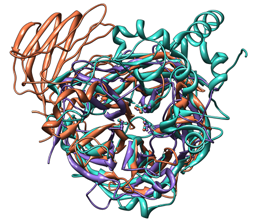
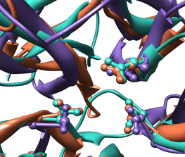
Comparison of glycoside hydrolases from different families. Invertase (family 32) is coral, arabinanase A (family 43) is purple, and levansucrase (family 68) is turquoise. Despite differences in sequence, substrate, and catalytic mechanism, the enzymes have similar overall folds (top) and a set of highly conserved acidic residues in the active site (bottom).

Glycoside hydrolases (GH) are a large, heterogeneous set of enzymes that catalyze the hydrolysis of certain bonds between sugars or between sugars and other moities. Based on sequence comparisons, these enzymes have been categorized into many families; see the CAZy web site for details.

This tutorial describes the creation of images to show structural similarities among certain members of GH families 32, 43, and 68. These enzymes were grouped into different families because their relationships were not clear from sequence information alone.

The approach described on this page is only one of many possibilities. Another is to generate static renderings with shadows.

On Windows/Mac, click the chimera icon. On UNIX, start Chimera from the system prompt:

unix: chimera

A basic Chimera window should appear after a few seconds; resize it as desired. Open the Command Line (choosing Tools... General Controls... Command Line is one way).

If you have internet connectivity, structures can be obtained directly from the Protein Data Bank. Choose File... Fetch by ID from the Chimera menu. In the resulting dialog, check the PDB ID option (if it is not already checked) and the option to Keep dialog up after Fetch. Fetch the PDB structures 1uyp, 1gyd, and 1oyg, in that order, and then Close the dialog. If you do not have internet connectivity, you can download the files 1uyp.pdb, 1gyd.pdb, and 1oyg.pdb into your working directory and then open them in that order as local files (with File... Open). (Or instead of opening these structures, one could just open the Chimera session that is saved below, but that would not be very instructive as to how the session was generated.)

Move and scale the structures with the mouse in the graphics window (and optionally, the Side View) as desired throughout the tutorial.

Some salient features of the structures:

PDB ID	enzyme	family	chains	conserved residues
1uyp	invertase, T. maritima	GH32	A-F	Asp17	Asp138	Glu190
1gyd	arabinanase A, C. japonicus	GH43	B	Asp38	Asp158	Glu221
1oyg	levansucrase, B. subtilis	GH68	A	Asp86	Asp247	Glu342

First, simplify the situation by deleting unwanted (for our purposes) portions of the structures such as extra chains and solvent, and then displaying just the alpha-carbon traces.

Command: delete #0:.b-f
Command: delete solvent
Command: chain @ca
Command: linewidth 3

Command: match #1:38.b,158.b,221.b@n@ca@c@o #0:17.a,138.a,190.a@n@ca@c@o
Command: match #2:86.a,247.a,342.a@n@ca@c@o #0:17.a,138.a,190.a@n@ca@c@o

The peptide backbone atoms of the conserved residues were used to match the structures. Another possibility would have been to use all atoms of these residues, as the residue types are the same across the different structures (match requires equal numbers of atoms from the two models being matched). Model 0 (invertase) was used as the reference structure for both pairwise matches. The number of points used for fitting and the resultant RMSD values are reported in the status line (transiently) and the Reply Log.

Alternatively, matchmaker could have been used to superimpose the structures. Instead of user-specified atoms, it uses the protein sequences and secondary structure to generate alignments. Superpositions similar to those obtained above with match can be obtained with the following:

Command: matchmaker #0 #1
Command: matchmaker #0 #2

Show the structures as ribbons, with only the side chains of the conserved residues shown in ball-and-stick form:

Command: ~disp
Command: ribbon
Command: sel #0:17.a,138.a,190.a #1:38.b,158.b,221.b #2:86.a,247.a,342.a
Command: disp sel

Command: repr bs sel
Command: ~sel

Command: ~ribbon #0:296-end.a

The background can be any color, but white is often good for publication.

Command: set bg_color white

When the background is white, depth cueing with dark shading looks strange. Open the Effects tool (Tools... Viewing Controls... Effects) and turn off depth cueing (uncheck the checkbox). A reasonable alternative would be to leave the depth cueing on, but change the depth cueing color. Clicking the color well brings up the Color Editor, allowing the depth cueing color to be set to white, or to No Color, which will automatically match the background. The amount of shading can then be adjusted by moving the clipping planes in the Side View.

Also in Effects, turn on silhouette edges to highlight boundaries and discontinuities, then Close the tool. Edges may look jagged, but supersampling will correct these within saved images.

Color the three models three distinguishable colors.

Command: sel #0
Actions... Color... all colors [pick a color]

Command: ~sel

The default ribbon style is flat. The edged and rounded styles are more three-dimensional.

Command: ribrepr rounded

The smoothness of curved surfaces in the stick, ball-and-stick, sphere, and ribbon molecular representations can be increased by raising subdivision quality in the Effects tool (Tools... Viewing Controls... Effects). Higher values increase smoothness but may slow performance. Values of 5.0-20.0 are reasonable for saved images, while lower values suffice for interactive use. 5.0 was used for the examples.

Similarly, the smoothness of molecular surfaces (not included in the examples) can be increased by increasing the vertex density in the surface attributes panel.

Straight edges may appear as tiny zigzags, especially against a white background. Supersampling gets rid of such jagged edges within saved images by making an initial image larger than that requested and then sampling it down to the final size. The level of supersampling can be controlled in the Image Setup preferences. The default value of 3x3, used for the examples, is generally sufficient for publication.

Resize the Chimera window to the desired aspect ratio, and then find view(s) suitable for the images. For the example images, a position was found that showed the overall structures well, and when scaled up (without further rotation) showed the conserved side chains well. The zoomed-out position was named overall, the scaled-up position was named closeup, and a session file named images.py was saved in the working directory:

Command: savepos overall
Command: scale 4
Command: savepos closeup
Command: reset overall
Command: save images

In this example, the session was saved in the overall position, but it could have been saved in another position (including one without a name) without any loss of information. It is generally prudent to save sessions for publication images, as this decreases the labor necessary if figures have to be redone. Often minor adjustments such as changing a color or displaying a different set of side chains will be required.

Later, the session can be restarted by opening images.py. If the models are moved around, the saved positions can be regenerated, for example:

Command: reset closeup

Before an image is saved, a particular position may need to be restored, for example:

Command: reset overall

Choosing File... Save Image brings up the Save Image panel. Editing the value for one dimension and then clicking in the field for the other dimension adjusts the latter automatically when Maintain current aspect ratio is on. The dimensions can be specified directly in pixels, or in units of length. If units of length, the number of pixels per unit can be controlled in the Image Setup preferences.

For example, to make an image for a single-column width of 85 mm (3.346 in) with a resolution of at least 300 dpi, possible approaches are to:

• set Units to pixels and Image width to at least 1004 pixels (3.346 x 300)
• set Units to inches, Image width to at least 3.346 in, and Pixels per unit (in the Image Setup preferences) to 300

The example images were saved in TIFF format; other possibilities are PNG, JPEG, PS (PostScript), and EPS (Encapsulated PostScript).

Labeling, stereo, and color space are discussed in the Image Tips.