
Tom Goddard April 2001
This page shows visualizations of 3D electron microscope data of a Drosophila chromosome. The aim is to reveal the packaging of the 30 nm chromatin fiber in the condensed chromosome. The data comes from Maria de Sousa Vieira formerly a researcher in John Sedat's group,
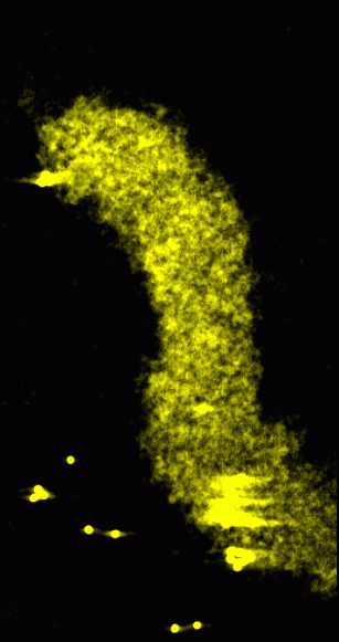
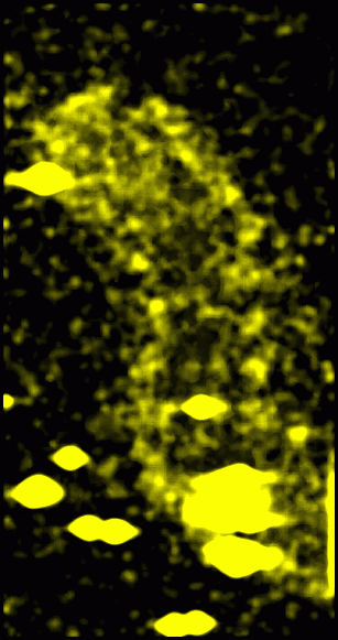
A subregion of the embryo11.xyzw volume is shown in below. The figures show the original data, smoothed data, ridges and valleys, and amplitude variation about the local mean. I don't see any evidence of a chromatin path in these figures. The data set used has negative density values outside the chromosome region suggesting that it has not undergone the post-back-projection processing. It would be worth looking at data that has undergone more tomography processing and at other samples.
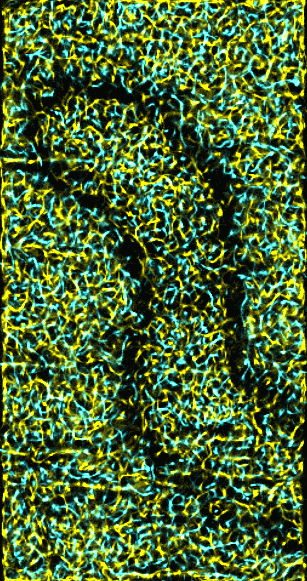
The subregion (168-423,0-487,0-63) of the embryo11.xyzw volume was used. The volume elements are spaced 2.62 nm apart. The 256 by 488 by 64 subregion is 671 nm in width, 1279 nm height and 168 nm in depth. The chromosome is roughly 200 nm wide. The images show transparent solids created using the volume viewer extension to Chimera. A transparency depth of 30 nm was used, and the brightness factor was typically set to .1-.5. The high threshold was usually left at the highest data value, and the low threshold was adjusted to produce the most informative image.

|
|
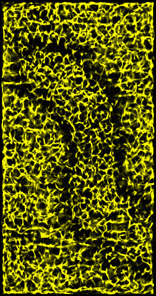
Figure 1: Original data rendered as a transparent solid. Crosseye stereo pair.
|
|
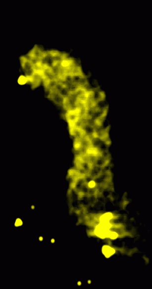
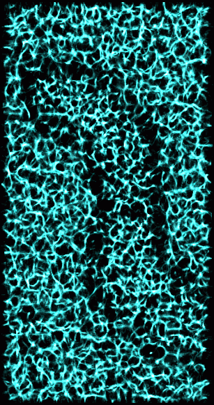
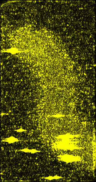
Figure 2: Transparent solid rendering of smoothed volume. The data was convolved with a Gaussian of linewidth 15 nm with the linewidth defined as the distance from -SD to +SD.
|
|
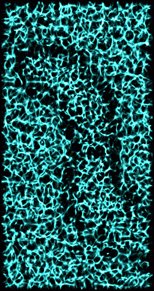
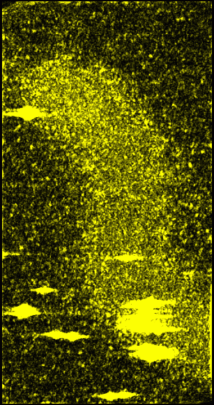
Figure 3: Ridges in 15 nm smoothed data. A ridge point is defined as one where most of the neighboring data values have lesser value -- that is, when you step away from a ridge you go downhill in most directions. This figure shows a derived volume which counts how many neighbors of each grid location are lower than the grid value. The neighbors of a grid point are the 26 grid voxels in a 3 by 3 by 3 box centered on the grid point. The brightest spots represent maxima where all 26 neighbors have lower value. The dimmer features have 18 or more neighbors of lower value. The derived volume is 2 grid points smaller along each axis because grid points on the edge of the original data box are not considered.
|
|
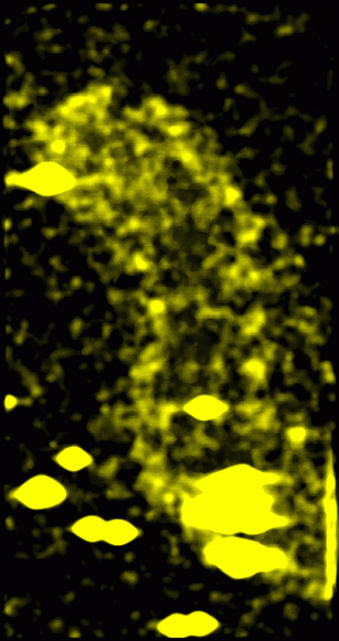
Figure 4: Valleys in 15 nm smoothed data. A valley point is defined like a ridge point in Figure 3, only most neighboring points have higher value. This shows the same derived volume as in Figure 3 with thresholds set to highlight valleys.
|
|
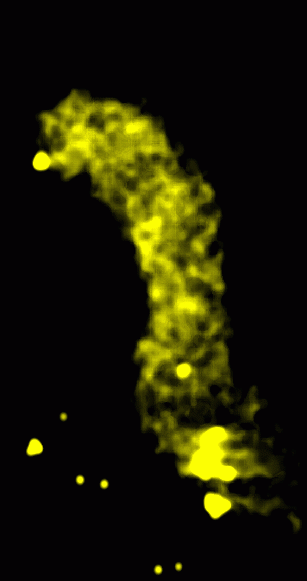
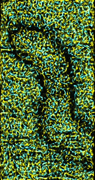
Figure 5: Ridges and valleys in 15 nm smoothed data.
|
|
Figure 6: Original data with 15 nm smooth version subtracted off and then absolute value taken. The idea behind this image is that the amplitude of the swing from peaks to valleys in each region might convey some useful information. This was found to be useful in analyzing unrelated data about the firing of neurons.
|
|
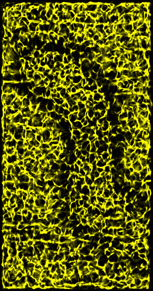
Figure 7: Original data with 15 nm smooth version subtracted off and then squared, convolved with a 15 nm Gaussian and square-rooted. This represents the standard deviation of data values from the mean in roughly 15 nm neighborhoods. It is a variation on the idea described in Figure 6.
Laboratory Overview | Research | Outreach & Training | Available Resources | Visitors Center | Search