This tutorial includes binding site analysis and comparison of related structures by superposition and morphing. Internet connectivity is required to fetch the structures 3w7f and 2zco.
The pathogenic organism Staphylococcus aureus makes a pigment called staphyloxanthin. The pigment imparts a golden color (hence aureus), but more importantly, contributes to virulence by protecting the bacteria from being killed by the host immune system. The S. aureus enzyme CrtM may be a good drug target because it catalyzes a key step in staphyloxanthin synthesis:
A cholesterol biosynthesis inhibitor blocks Staphylococcus aureus virulence. Liu CI, Liu GY, Song Y, Yin F, Hensler ME, Jeng WY, Nizet V, Wang AH, Oldfield E. Science. 2008 Mar 7;319(5868):1391-4.We will view and compare different structures of this enzyme.
Start Chimera by clicking or doubleclicking the Chimera icon
![]() (depending on its location).
Typically, this icon will be present on the desktop.
The Chimera executable can also be run from its
installation location (details...).
(depending on its location).
Typically, this icon will be present on the desktop.
The Chimera executable can also be run from its
installation location (details...).
A splash screen will appear, to be replaced in a few seconds by the main Chimera graphics window or Rapid Access interface (it does not matter which, the following instructions will work with either). If you like, resize the Chimera window by dragging its lower right corner.
Show the Command Line (Tools... General Controls... Command Line). Choose Favorites... Add to Favorites/Toolbar to place some icons on the toolbar. This opens the Preferences, set to Category: Tools. In the On Toolbar column, check the boxes for:
|
 |
 |
 |
|
 |
Fetch a structure from the Protein Data Bank and use the ribbons preset:
Command: open 3w7f
Menu: Presets... Interactive 1 (ribbons)
| active site |
|---|
 |
Command: delete :.bMove and scale structures using the mouse and Side View as desired throughout the tutorial.
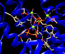
The enzyme combines two 15-carbon molecules of farnesyl pyrophosphate to form a 30-carbon lipid. This structure contains farnesyl thiopyrophosphate, which differs from the substrate by having a sulfur in the place of one oxygen. Sulfur atoms are shown in yellow, phosphorus orange, oxygen red, and nitrogen blue. Label the ligand residues:
Command: rlabel ligandIn this structure, the farnesyl thiopyrophosphate molecules are named FPS. Three magnesium ions help to offset the negative charges on the phosphates. The ions are shown as greenish spheres; clicking into the Chimera window and hovering the mouse cursor over each shows information in a pop-up balloon. Metal coordination bonds from FPS, water, and the protein are shown with dashed purple lines. Lines drawn to indicate interactions other than covalent bonds are called pseudobonds. Hovering the cursor over a pseudobond or bond shows balloon information about its end atoms and length.
Delete the water, label residues with displayed sidechains, and place the labels near α-carbons instead of residue centroids:
Command: del solventWater could be included in the various analyses, but is removed here to simplify the tutorial.
Command: rlab @/display
Command: setattr m residueLabelPos 2
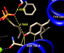
It looks like several sidechains could be donating hydrogen bonds to phosphate oxygens. (Although the structure does not include hydrogens, we know they are there!)
One of the displayed residues is Ser 21. To measure a distance:
The distances seem consistent with hydrogen bonds. However, rather than measuring many distances and trying to remember the appropriate hydrogen-bonding distances for different types of atoms, just use FindHBond. We will limit the search to H-bonds involving the FPS residues:
Command: ~hbondFind Clashes/Contacts is similar to FindHBond but can also identify nonpolar interactions:
One might simply want a list of the interacting residues rather than the details of each atomic contact. A list of the selected residues can be saved. First, deselect the ligand residues and ions, leaving the protein residues selected:
Command: ~sel ligandOpen the Selection Inspector by clicking the magnifying glass icon
Command: ~sel ions
 near the bottom right corner of the main window.
It reports that 26 residues are selected.
Click its Write List... button
(or choose Actions... Write List from the main menu).
In the resulting dialog, indicate that selected residues
should be written. Click Log to write the list to the
Reply Log instead of to a file.
near the bottom right corner of the main window.
It reports that 26 residues are selected.
Click its Write List... button
(or choose Actions... Write List from the main menu).
In the resulting dialog, indicate that selected residues
should be written. Click Log to write the list to the
Reply Log instead of to a file.
Amino acid torsion angle values can be viewed in the Selection Inspector. Focus on Tyr 248:
Command: focus :248Ctrl-click to pick any atom or bond in Tyr 248. This will replace (clear) any pre-existing selection. Open the Selection Inspector again if it is not already open. Inspecting Residue (instead of Atom) shows that the sidechain angles chi1 and chi2 in this residue are approximately –107° and –142°, respectively. The backbone angles phi and psi are also given. Close the Selection Inspector.
| clash checking |
|---|
 |
We will set up clash checking and rotate the sidechain interactively.
Command: disp :248 z<4
Use whichever method you prefer to rotate the bond. As the sidechain moves, yellow pseudobonds show any clashes, and the distance monitor updates automatically. The sidechain is fairly constrained; only chi1 angles of approximately –(100–120)° avoid clashes if only that bond is rotated. The sidechain can be frozen in a new position, but for tutorial purposes, simply restore it to its original position: in the Adjust Torsions dialog, click the entry under Bond to show a menu. In that menu, choose Revert (move back to original position) and then Deactivate (make the bond no longer rotatable). Close the torsion dialog.
Click the Find Clashes/Contacts icon to bring the dialog to the front and Close it to halt clash checking.
Next, we will compare the conformation of Tyr 248 in the structure to tyrosine rotamers from a library. This will indicate whether the sidechain is in a frequently observed conformation and whether other conformations might also fit into the structure.
With part of Tyr 248 still selected (if not, Ctrl-click to
to select any of its atoms or bonds), start
Rotamers by clicking its icon
![]() .
Click OK to show TYR
rotamers from the Dunbrack 2010 backbone-dependent library.
The rotamers are shown in the wire representation and listed in another dialog.
.
Click OK to show TYR
rotamers from the Dunbrack 2010 backbone-dependent library.
The rotamers are shown in the wire representation and listed in another dialog.
The rotamer dialog reports chi1 and chi2 angles and probabilities from the library based on the residue's backbone conformation. Choosing a row (or rows) in the rotamer dialog displays just the corresponding rotamer(s). From the chi angles in the dialog and the 3D display, it is evident that none of the rotamers match the conformation in the structure. Other than the backbone angles, the probabilities given in the dialog do not take into account any interactions specific to this structure. However, the rotamer dialog is integrated with clash and H-bond detection. Choose Columns... Add... Clashes and click OK to use the default settings; repeat with Columns... Add... H-Bonds.
The new columns show that each rotamer forms several clashes but no hydrogen bonds. We showed above that Tyr 248 H-bonds with the ligand and avoids clashes, which may compensate for its nonrotameric (presumably strained) conformation.
A sidechain can be replaced with a chosen rotamer. With a single rotamer shown, either click OK in the rotamer dialog to replace the sidechain with that rotamer and remove the others, or simply Close the dialog to remove the rotamers without replacing the sidechain. Although not done in this case, rotamers can be shown for a different amino acid type than in the structure, allowing for virtual mutations.
Unlike Tyr 248, Tyr 41 closely resembles the highest-probability tyrosine rotamer given its backbone angles. If you like, focus on Tyr 41, select one of its atoms or bonds, and use Rotamers to show and evaluate rotamers of tyrosine or some other amino acid at that position.
Clear the selection, unlabel the residues, zoom back out, and remove the distance pseudobonds:
Command: ~sel
Command: ~rlab
Command: focus
Command: ~dist
FPS and the natural substrate both have a highly polar/charged “head” and a long hydrocarbon “tail.” The enzyme pocket is very large and deep, as needed to accommodate two of these molecules.
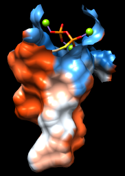
A surface representation is best for showing the shape of the pocket. Choose Presets... Interactive 3 (hydrophobicity surface) from the menu to display a molecular surface color-coded by amino acid hydrophobicity. This preset colors the surface ranging from dodger blue for the most polar residues to orange red for the most hydrophobic, with white in between.
As one might expect, the mouth of the pocket near the phosphates and ions is mostly polar, while the rest of the pocket is largely hydrophobic. However, the pocket is so deep that it is hard to see when the whole surface is shown. Restricting the surface display to the pocket region allows it to be viewed from the outside, as shown in the figure.
Hide the ribbon and the protein atoms, then show only surface near the ligand:
| pocket surface |
|---|
 |
Command: ~ribbon
Command: ~disp protein
Command: sop zone #0 ligand 5.0 max 1
The sop (“surface operations”) command limits the display of surface #0 to a 5.0-Å zone around the ligand and shows only the largest resulting fragment. Without max 1, a few additional disconnected shards of surface would be shown. If you like, try different cutoff values; the figure shows results for a cutoff of 4.7 Å.
Amino acid hydrophobicity is one example of an attribute. Another attribute commonly used in structure analysis is atomic B-factor. B-factor values indicate which parts of the structure are more or less flexible or disordered.
Display all atoms by choosing Presets... Interactive 2 (all atoms) from the menu. Now the ligand atoms are shown as spheres and the protein as wires. Show the protein as sticks:
Command: repr stick protein
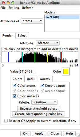 |
In the Render dialog, switch from atoms to residues and show the histogram for the attribute kdHydrophobicity, the Kyte-Doolittle hydrophobicity of amino acids. This is the same attribute as used by the surface preset, but different coloring schemes can be applied. Larger positive values correspond to more hydrophobic residues, negative values to hydrophilic residues. The No-value color pertains to residues without Kyte-Doolittle hydrophobicities, namely any that are not amino acids (such as the ligands in this structure). The colors can be changed as described above. Apply coloring by hydrophobicity if you like, then Close the dialog.
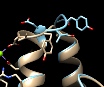
Comparing different structures of a protein is another way to evaluate flexibility. We have been viewing a structure bound to substrate analogs, 3w7f. A structure of the same enzyme without ligands is also available. Fetch the “empty” structure and apply the ribbons preset:
Command: open 2zcoNow the first structure is tan and the new structure is sky blue, as shown in the Model Panel (Tools... General Controls... Model Panel).
Command: preset apply int 1
The structures are in completely different positions, so the next step is to superimpose them. This is easily accomplished with MatchMaker or its command equivalent:
Command: mm #0 #1 show trueMatchMaker first generates a sequence alignment using residue types and secondary structure (tries to align helix with helix and strand with strand), then fits the sequence-aligned residues in 3D by pairing their CA atoms. The show true option displays the sequence alignment. By default, the fit is iterated so that far-apart pairs are not included in the final match. This allows the most similar parts to superimpose more tightly and the dissimilar parts to stand out. Final match statistics are reported in the Reply Log, and the pairs used in the final fit are shown with light orange boxes on the sequence alignment. The RMSD histogram above the sequences shows spatial variability, calculated as the root-mean-square deviation among the CA atoms of residues associated with each column. In this case (only two structures), the RMSD value is the same as the CA-CA distance.
| different loop conformations |
|---|
 |
The structures are highly similar except for the loop at approximately residues 52-56; you can see residue numbers by clicking into the sequence alignment window and hovering the cursor over the corresponding one-letter codes. Click any part of the light orange boxes to select all the residues used in the final fit; these form the common core, the most conformationally similar parts of the structures. The selection can be inverted if you want to do something to the less similar parts, for example:
Command: sel invertMorphing involves calculating a series of intermediate, interpolated structures between the original input structures. In Chimera, the series of structures is treated as a trajectory that can be replayed, saved to a coordinate file, or saved as a movie using MD Movie.
Command: disp sel & protein
Command: ~sel
Start the morphing tool:
Menu: Tools... Structure Comparison... Morph ConformationsClick Add... and in the resulting list of models, doubleclick to choose #0, #1, and #0 again, corresponding to a morph trajectory from the ligand-bound structure to the empty structure and back. Close the model list. In the main Morph Conformations dialog, set the Action on Create to hide Conformations, and then click Create.
The progress of the calculation is reported in the status line. When all the intermediate structures have been calculated, the input structures are hidden, the trajectory is opened as a third model (#2), and the MD Movie tool appears. The trajectory can be played continuously or one step at a time by clicking buttons on the tool, or a frame number can be entered directly. If the MD Movie playback dialog becomes obscured by other windows, it can be raised using its instance in the Tools menu (near the bottom of the menu, below the horizontal line).
The initial display of the morph trajectory is as ribbons rather than all atoms, but all atoms that are present in both input structures are also present in the morph. Their display can be controlled just as in any other structure, for example:
Command: disp #2:52-56Ligand residues were only present in one of the structures, so they are not included in the morph trajectory. However, part or all of the original structures can be displayed along with the trajectory. Display of the other models can be re-enabled by checking the S(hown) boxes in the Model Panel (Tools... General Controls... Model Panel) or with a command, for example:
Command: modeldisp #0Then, to show only the ligand residues and ions from that model:
Command: ~ribbon #0In this case, the secondary structure does not change much between the input structures. When conformational differences are larger and ribbons will be displayed, one may want to re-evaluate the secondary structure at each step of the trajectory. That can be done by putting the command ksdssp in a per-frame Chimera script in MD Movie. Such scripts also allow performing actions (such as showing/hiding a ligand) at specific steps in the trajectory.
Command: show :fps,mg
The Morph Conformations page lists a few additional example systems.
When finished enjoying the morph trajectory, choose File... Quit from the menu to exit from Chimera.