Last revised October 22, 2012.
Here is a tour of methods for displaying volume data sets using interactive graphics program UCSF Chimera. Data for example images comes from
|
|
|
|
|
| Segment mouse mode (video) | Segment and fit (video) | Box around marker | Plane topography |
| 
|
| 
|
| Mask to surface | Rotated subregion | Plane display | Split map by color |
| 
| 
| 
|
| Erase outside sphere | Zone display | Slicing and capping | Slab clipping |
| 
| 
| 
|
| Icosahedral slice | Erase octant | Hand erasing | Subregions |
| 
| 
| 
|
| Place spherical markers (video) | Find symmetry axis | IMOD surfaces | Symmetric fitting |
| 
| 
| 
|
| Fit map in map | Fit model in map | Place markers | Icosahedral cage |
| 
|
| Smooth mask (video) | Binning |
| 
| 
| 
|
| Hide dust | Median filter | Fourier transform | Gaussian smoothing |
|
| Local correlation (video) |
| 
| 
| 
|
| Degree of symmetry | Measure volume | Path length | Shell radius |
| 
| 
| 
|
| Color connected surface | Color zone | Radial coloring | Electrostatic potential |
|
| Color by density value |
| 
| 
| 
|
| Morph map | Ambient occlusion lighting | Box face capping | Square mesh |
| 
| 
| 
|
| Close boundary holes | Surface smoothing | Multiple contour levels | Display styles |
This web page is being developed. Some topics not yet covered are:
    molmap - map computed from molecule
    angle-dependent transparency
    silhouette edges with transparency
    single layer transparency
    mask slab, nuclear envelope
    per-pixel surface color
    fly command
    measure correlation coef
    split by zone around marker
    Laplacian filter
    invert, scale, shift filter
    resample subregion (update)
    distance to surface
    select atoms outside surface
    determine map symmetry
    multiscale
    better meshes, smoothing, refine, subsample
    hand docking, constrained move
    values at atom positions
    origin and scaling
    path tracing
    tube marker interpolation
    writing volumes
    superposition tricks - multiple data copies
    lighting
    transparency with PDB model
    time series
    volumetric rendering, maximum intensity projection
    scale bar
    file format list
    afm data
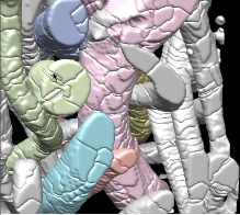
Segment mouse mode | (June 16, 2010, version 1.5 daily build, details, video) |
Density maps can be segmented by clicking on regions with the mouse and dragging to control the extent of the region. The dragging sets a density level and connected density above that threshold forms a region. Regions obtained by watershed segmentation are shown and joined using these mouse actions. To turn on the mouse mode first display the Segment Map dialog,
Tools / Volume Data / Segment Map
press the Options button, and enable
Group with mouse [button 3]
Button 3 means the right mouse button of a 3-button mouse. Select the map to segment in the Segment map menu at the top of the dialog and click on density map (using button 3). The first click calculates and displays the watershed regions and can take some time. Then click and drag on specific regions to group them into segmented objects. Groups will be indicated by color, and new regions will not extend into already grouped regions. Releasing the mouse button shows the objects touching the last segmented object. Clicking on the background will show the remaining ungrouped regions. A second click on the background will show all regions, grouped and ungrouped.
This method was developed for rather well separated objects touching in small places (bacteria in termite gut). It will be very slow for more than 100,000 watershed regions (local maxima) so smoothing the volume data beforehand may be necessary to reduce the number of regions. On Mac OS 10.6 poor system graphics driver memory management makes the region display unusably slow for more than 5000 displayed regions.
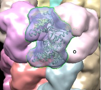
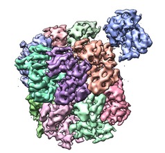
Segment and fit | (June 16, 2010, version 1.5 daily build, details, video) |
Density maps can be segmented by computing watershed regions of and grouping them using according to overlap with watershed regions of smoothed copies of the map. This method works well on single-particle EM reconstructions of molecular assemblies.
Open the map and set a desired contour level. Only parts of the map above the displayed contour level will be segmented. Press the Segment button on the Segment Map dialog.
Tools / Volume Data / Segment Map
Colored regions will be shown. If the aim is to make the regions correspond to individual molecules and the computed regions are too small, pressing the Group button will perform another round of smoothing and grouping to produce fewer regions. The Ungroup button will make smaller regions undoing the previous smoothing round. If regions are selected with the mouse (ctrl-click and shift-ctrl-click) then the Group and Ungroup buttons instead just join or split apart the selected regions.
The default settings in the options panel (Options button) do three rounds of Gaussian smoothing with standard deviations 1, 2, and 3 grid spacings to group the watershed regions of the unsmoothed map. A watershed regions is the set of points that reach the same local maximum of the density map following a steepest ascent walk.
This method will be very slow for more than 100,000 watershed regions (local maxima). For very high resolution maps smoothing the volume data beforehand may be necessary to reduce the number of regions. On Mac OS 10.6 poor system graphics driver memory management makes the region display unusably slow for more than 5000 displayed regions.
To fit a molecular model into a segmented region, show the Fit to Segments dialog
Tools / Volume Data / Fit to Segments
Select the molecule file from the Structure to fit menu if it is in the same directory as the density map. Or you can open the structure using the normal Chimera File / Open... dialog and then select it in the menu. Then select the region to fit to (ctrl-click on the region), and press the Fit button. This aligns the principle axes of the molecule with those of the region density and then does a local rigid optimization.
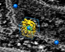
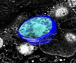
Box around marker | (2001, version 1.0, details) |
To limit map display to a box around a selected marker use the volume dialog Atom Box panel, shown using volume dialog menu entry
Features / Atom box
Enter a padding value which is the distance from the center of the selected marker to the edge of the desired box and press the Box button. This restricts the map display to that box. The subvolume can be saved to a new map file with volume dialog menu entry File / Save Map As....
See the marker placement description for how to create markers. If more than one marker is selected when the Box button is pressed then a single subregion is shown enclosing all the markers with minimum distance from the boundary to any marker equal to the padding value.
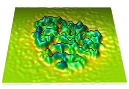
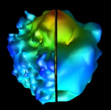
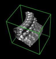
Plane topography | (November 2007, version 1.2475, details) |
The topography command creates a surface from a volume plane where the height of the surface above the volume plane is proportional to the data values. After displaying a single plane of volume data, the following Chimera command
topography #0 height 10
will create the surface. To enter the command show the Chimera command line with menu entry Favorites / Command line. The #0 parameter is the volume model number. The model numbers are listed in the Model Panel dialog, shown with menu entry Favorites / Model Panel. The height value specifies the height of the surface from minimum data value to maximum volume data value. It is specified in the length units associated with the map, such as Angstroms.
By default the surface is colored red to blue from lowest to highest points. This and several smoothing / interpolation capabilities are controlled by additional command options that are described in the User's Guide. Different color schemes can be applied using the color by height capabiliy of the Surface Color tool (menu entry Tools / Volume Data / Surface Color).
Mask to surface | (October 2007, version 1.2467, details) |
You can extract part of a map bounded by a surface using the mask command. The surfaces can be drawn in another software package IMOD and imported into Chimera. Or surfaces created within Chimera such as the contour surface of a Gaussian filtered map can be used.
Display the command line with menu entry
Favorites / Command line
then type a command such as
mask #0 #1
to copy part of volume #0 bounded by surface model #1. Model numbers start at zero and new models are assigned the next available number. The model numbers are listed in the Model Panel dialog, shown with menu entry Favorites / Model Panel. To mask to just a single surface object in and IMOD segmentation use a command such as
mask #0 sel axis 1,0,0
This command copies part of volume #0 within the selected surface projecting along the x axis. The surface object is selected using the left mouse button with the ctrl key held down. The projection axis (default z) effects how holes in the surface are handled. Points within the surface when viewed along the projection axis are taken.
The new volume with zeros outside the surface can be saved to a file using volume dialog menu entry File / Save map as.... The map will usually be smaller than the original map unless the fullmap option is used with the mask command. The origin will be specified in the new volume file so that it will align with the original map.
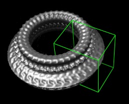
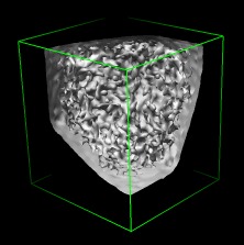
Rotated Subregion | (September 2007, version 1.2443, details) |
You can extract part of a map that is not aligned with the axes of the original map. This is useful for chopping out objects in tomograms that are not aligned with the map axes. Open the map, then use the Subregion Selection panel of the volume dialog (in the Features menu). Turn on Select subregions using button 2 and drag a green selection box around the part of the map of interest with mouse button 2. Then click the
Rotate selection box
checkbutton. This freezes the map (and any other models) so that you can rotate only the green outline. To move the green outline box side to side click and drag outside the bounds of the box with mouse button 2. Hold down the shift key at the same time to move the box in the z direction. Press the
Resample
button to create a new volume data set with those bounds. The data can be saved to a separate file using volume dialog menu entry File / Save map as.... The rotation is saved in MRC and Chimera format map files and will align with the original data when opened in subsequent sessions. Uncheck the Rotate selection box button to allow normal rotation of all models.
This procedure interpolates (resamples) the original map on a new grid with voxel spacing given by the Resampling voxel size listed in the subregion panel of the volume dialog. You may wish to change that to a value smaller than the original map voxel size to avoid reducing resolution.
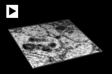
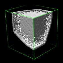
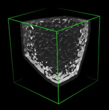
Plane display | (July 2007, version 1.2430, details) |
Single planes can be displayed with gray scale rendering, frequently useful for tomography data. Use the Planes panel of the volume dialog shown with volume dialog menu entry
Features / Planes
Turn on the plane checkbutton next to the plane number and slider. Planes perpendicular to the z, y, or x axes can be displayed using the axis menu and a slab containing more than one plane can be shown using a depth entry greater than 1. The Play button cycles through the planes, reversing direction when the end planes are reached.
Plane display uses solid rendering and sets the displayed subregion to show just the desired plane. The yellow line on the histogram controls the brightness of different data values.
Split Map by Color | (October 2007, version 1.2458, details) |
A map colored with the color zone tool can be split into separate maps, one for each color. The splitting is done using the
Split Map
button on the color zone dialog. The splitting creates a separate map for each color zone color of the map currently displayed in the volume viewer dialog. If the displayed map is a subregion then the newly created maps include just that subregion. The new maps always includes all data from the subregion even if the original map was displayed with subsampling. The new maps are given names with 0,1,2,... appended to the original map name. The original map is undisplayed although it remains open. The map with 0 appended is the uncolored part of the original map (i.e. outside of the color zone) and the other colors are ordered randomly. The new maps can be saved (one at a time) to files using volume dialog menu entry File / Save Map As....
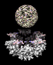
Erase Outside Sphere | (November 2005, version 1.2186, details) |
A map can be set to zero outside a sphere to extract a spherical piece. This is useful for virus particles. This uses the Volume Eraser tool, menu entry
Tools / Volume Data / Volume Eraser
Adjust the sphere position with the mouse, and sphere radius with the slider in the Volume Eraser dialog. To set the data values outside the sphere to zero use keyboard accelerator eo ("erase outside"). Use of keyboard accelerators is turned off by default. Turn them on with menu entry
Tools / General Controls / Accelerators On
Then type eo in the main graphics window. You do not press the Enter key. This keyboard accelerator is currently the only way to erase outside a sphere. There is no equivalent dialog button or Chimera command.
The image shows the dodecahedral penton particle from human adenovirus type 3, EM Database entry 1178
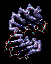
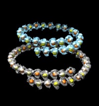
Zone display | (August 2005, version 1.2154, details) |
Volume data can be displayed just within a specified distance of selected atoms or markers. Check the Region switch at the top of the volume viewer dialog (menu entry Tools / Volume Data / Volume Viewer). This expands the dialog to contain extra buttons. Select atoms from an already opened PDB molecule with the mouse by holding down the ctrl key and dragging a box or clicking individual atoms. Then press Zone. This restricts display of the volume surface to only show parts within 2 angstroms. The range can be changed using the slider below the Zone button.
Atoms can be selected in many different ways. Menu Select / Chain / A can be used to select chain A. To select a single residue ctrl-click on an atom of the residue then press the up arrow key to extend the selection to the containing residue. The Sequence dialog (menu Tools / Structure Analysis / Sequence) shows the amino acid sequence using one letter codes that can be selected to select ranges of residues.
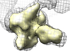
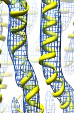
The image shows an RNA / DNA hybrid, the base pairs at both ends being RNA and the 8 base pairs in the middle being DNA. The crystallographic density map used to solve this structure is shown around just one strand of the double helix. (PDB 100d and denisty map from the Uppsala Electron Density Server).
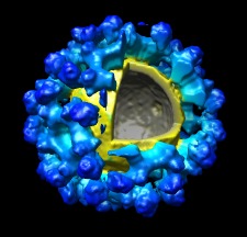
Slicing and capping | (August 2005, version 1.2154, clip and cap details) |
A map can be sliced in half with a plane at an arbitrary angle using
Tools / Depiction / Per-Model Clipping
Turn on the Enable clipping switch in the dialog that appears. The cut plane can be moved by turning on the Adjust clipping with mouse switch near the bottom of the Per-Model Clipping dialog. The hole left by slicing a surface can be covered with a cap using
Tools / Depiction / Surface Capping
Turn on the Cap surfaces at clip planes switch in the surface capping dialog. The cap can be displayed as mesh and with a different color using dialog settings. Shown is a ribosome bound to tmRNA (a combined tRNA / mRNA sequence) (EM database entry 1122). This sequence unclogs ribosomes blocked by defective mRNA.
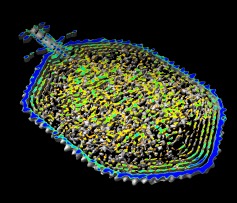
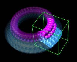
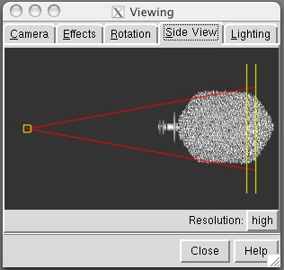
Slab clipping | (August 2005, version 1.2154, clip and side view details) |
|
| 
| 
|
A slab of a volume data set can be displayed using
Tools / Depiction / Per-Model Clipping
Turn on the Enable clipping switch and the Use slab mode switch. The location of the slab in the data set can be changed by turning on the Adjust clipping with mouse switch and dragging with the mouse. Slabs parallel to the screen can be obtained with
Favorites / Side View
This shows a view of the data from the side. The small yellow square at the left represents your eye. The two vertical yellow lines are the near and far clip positions. These can be dragged with the left mouse button so they are close to one another. Drag the left (near plane) line with the middle button to move both lines together. Drag the right (far plane) line with the middle button to change the separation between the planes (thickness of slab).
A 5 angstrom thick slab of Phage T4 is shown colored by density values (EM database entry 1075). Yellow is low density and blue is high density using the Surface Color tool. Concentric layers of the virus DNA are visible.
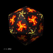
Icosahedron slice | (November 2005, version 1.2186, icosahedron and surface color and origin details) |
|
|
| Movie |
Icosahedral and spherical slices of a density map can be shown using the Icosahedron Surface tool and the Surface Color tool, menu entries
Tools / Higher-Order Structure / Icosahedron Surface
Tools / Volume Data / Surface Color
This is intended for looking at sections of icosahedral virus particles. The icosahedron surface tool displays a surface linearly interpolated between an icosahedron and a sphere, and the surface color tool colors that surface according to density map values. Use the Show button on the icosahedron surface tool to create the surface. Set the subdivision factor to 64 to produce a fine mesh. Colors are assigned to individual surface vertices so fine mesh is needed to see short-range density variations. Use the Open map data... button on the Surface Color tool to select the density map, press the Set full range colormap values button, and then the Color button.
If the density map is not centered at the origin (where the icosahedron is centered) then you can recenter it. Show the Volume Viewer dialog.
Tools / Volume Data / Volume Viewer
Select the density map from the Data menu at the top of the volume dialog. Then use volume dialog menu entry
Features / Origin and Scale
and change the origin values. The origin specifies the location of the corner of the map in xyz coordinates. To place the center of the map at (0,0,0) position the corner at -(voxel size)*(map size - 1)/2. Press the Enter key in one of the Origin entry fields or press the Show button at the bottom of the dialog to use the new origin.
Rice dwarf virus (EM database entry 1060). Movie shows density at varying radii.
Erase Octant | (November 2005, version 1.2186, details) |
To erase a box subregion of a volume data set, first draw the box using the volume viewer subregion selection capability and then erase the data in the box using keyboard shortcut eb. Here are details. First open the data. Next use volume dialog menu entry Features / Subregion selection which adds some buttons to the volume dialog. Click on the Select subregions using button 2 checkbutton, and then drag a box in the graphics window. The 3-dimensional green outline box can be adjusted by dragging faces of the box (not edges and not vertices) with mouse button 2. Now activate use of keyboard shortcuts with menu entry:
Tools / General Controls / Accelerators On
Now type "eb" to erase the volume data in the green subregion box. Erasing causes a writable copy of the data set to be created. See the Volume Eraser documentation in the User's guide for more details.
The data shown is kelp fly virus (EM database entry 1154) and it has been radially colored.
Hand Erasing | (November 2005, version 1.2186, details) |
|
| 
|
The volume eraser tool lets you erase data within a sphere. The sphere can be moved and resized, data values inside the sphere can be set to zero. Start this tool with menu entry
Tools / Volume Data / Volume Eraser
The sphere can be dragged using the mouse ctrl button 3. Pressing the Erase button sets the data values inside the sphere to zero. The first erasure causes a writable copy of the data set to be created. The modified data can be saved using the volume dialog menu entry File / Save Map As.... There is no undo capability.
The data shown is part of rice dwarf virus (EM database entry 1060) and it has been colored with the color zone tool.
Subregions | (August 2005, version 1.2154, details) |
|
| 
| 
|
| Before cropping | After cropping |
Display can be restricted to a subregion of a data set using the volume viewer dialog. The dialog is shown whenever you open a volume data set or you can use menu entry
Tools / Volume Data / Volume Viewer.
The checkbuttons at the top of the volume dialog expand the dialog to show more features. Click the Region checkbutton at the top. Then turn on Select subregions using button 2. Now drag a box over the desired subregion of the data set in the graphics window and press the Crop button. Subregions are constrained to be boxes aligned with the volume data axes. You can adjust the green outline box by dragging any of the 6 faces with mouse button 2.
The image shows a bacterial toxin pneumolysin that forms pores as large as 26 nm in cholesterol containing membranes to kill cells. (EM database entry 1107). The colored image used two copies of the data set, one colored transparently, with coloring by height using the Surface Color tool.
Smooth mask | (October 2012, version 1.7, details, video) |
The vop falloff command smooths the boundaries of masked maps by replacing each value outside the mask by the average of its 6 nearest neighbor values. The averaging is repeated for 10 iterations although a higher number can be chosen for smoother appearance or lower number for quicker falloff outside the mask. For a map with id number 2 the command would be
vop falloff #2 iterations 10
To show the Chimera command line use menu entry
Favorites / Command-line
The command will create a copy of the map with smoothing applied. Details of how the appearance and falloff boundary thickness vary with the number of iterations have been illustrated with a simple case of masking a uniform density to a sphere. For the default 10 iterations the drop off to half density occurs over a distance of about 0.7 grid points.
Binning | (June 2009, version 1.4, details) |
The binning filter averages volume data values in 2 by 2 by 2 boxes reducing the size of the map by 2 in each dimension. This increases the signal to noise ratio, especially useful for noisy tomography data. Larger bin sizes can be used. Show the volume filter dialog with
Tools / Volume Data / Volume Filter
select Filter Type "Bin" and press the Filter button. The filter is applied on the currently highlighted map in the volume dialog and creates a new map.
The new map only contains the displayed subregion of the original map. To make the new map cover the entire original map press the Options button and turn off "Displayed subregion only". For large maps that do not fit in memory, the new map may not display with a warning about memory allocation failing. The new map is still valid but only a smaller region can be shown. The full binned map can be saved with the volume save command (e.g. "volume #0 save ~/Desktop/binned.mrc") or Volume dialog File / Save Map As menu entry. This does not require the full original map to fit in memory since only a single data plane is read and written at a time.
The binning can be done with the vop command (e.g. "vop #0 bin binsize 3") instead of the volume filter dialog.
Hide Dust | (January 2009, version 1.4, details) |
The hide dust tool hides small surface blobs. It does not create a new volume data set. It provides a clearer view of large connected structures. Use menu entry
Tools / Volume Data / Hide Dust
choose the desired surface and press the Hide button. Disjoint surface blobs smaller than the size limit are hidden. The size is the maximum size along the x, y and z axes in the surface coordinate system. Adjusting the slider automatically updates the surface display for the new size limit. The Options button shows a panel allowing other size measures: hiding the smallest N percent of blobs, or hiding blobs enclosing less than a specified volume. Hide dust works on any surface including ones not derived from volume data.
Median Filter | (January 2009, version 1.4, details) |
Median filtering reduces noise while maintaining edges. Use menu entry
Tools / Volume Data / Volume Filter
choose filter type Median 3x3x3, press the Filter button. If more than one volume data set is open then the highlighted one in the volume viewer dialog will be filtered. A new volume data set is created and the original volume is hidden. Each data value is replaced by the median of the 27 nearest values (3 by 3 by 3 box). The iterations parameter allows applying the median filtering operation more than one time in succession. Three iterations is frequently useful. The grid points on the boundary of the new volume have value 0. The new map can be saved with volume dialog menu entry File / Save Map As....
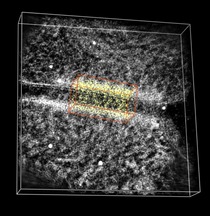
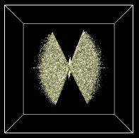
Fourier Transform | (October 2007, version 1.2458, details) |
To display the Fourier transform of a map use menu entry
Tools / Volume Data / Fourier Transform
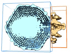
This creates a new map that is the Fourier transform (FT) of the volume dialog active map. The original map remains open in Chimera but is undisplayed. The new map contains only the magnitudes of the Fourier coefficients because Chimera does not work with complex value maps. The outline box for the FT map is displayed. Values near the edge represent high frequency components while those near the center represent low frequency components. The FT map is centered at the center of the original map and its size is scaled to match the enclosed volume of the original map. The physical units along the axes are reciprocal length so their scaling relative to Chimera length coordinates is not meaningful. If the original map grid plane spacing is not the same for x, y, and z axes then the FT map box will not be a cube. The longest dimension of the FT box will correspond to the smallest grid plane spacing.
The FT map can be used to assess the amount of oversampling in the original map (non-zero Fourier coefficients fill only a small sphere). The image shows the Fourier transform of tomography data (EMDB 1155) with the missing wedge caused by limited tilt angles in data acquisition.
Because the FT map does not include phases, applying a second FT will not reproduce the original map. Therefore erasing frequency components (with volume eraser) cannot be used as a selective filtering technique.
The FT map zero wavelength coefficient is set to zero. That is done because its value is usually so large that it makes the histogram display in the volume dialog uninformative because of the empty range of values between the zero term and all other terms covers almost the entire histogram.
Gaussian Smoothing | (October 2007, version 1.2454, details) |
A map can be smoothed by convolution with a Gaussian of specified width. Use menu entry
Tools / Volume Data / Volume Filter
or in Chimera 1.3 or older versions
Tools / Volume Data / Gaussian Filter
Enter the width of the Gaussian and press the Filter button to create a new map. The width is specified in the same units as the map (typically Angstroms or nanometers or grid planes). Chimera only keeps track of the spacing between grid planes for the map, not the name of the physical units. To see grid plane spacing used for the map use volume dialog menu entry Features / Origin and Scale and look at the voxel size. The Gaussian width specified in the filtering dialog is one standard deviations. The filtering is applied to the map that is shown in the volume dialog at the time the Filter button is pressed.
The original map remains open in Chimera but is undisplayed. Typically the contouring level will need to be adjusted on the smoothed map to see features of interest even though the Gaussian kernel is normalized to 1. The new map can be saved with volume dialog menu entry File / Save Map As....
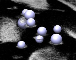
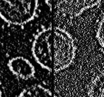
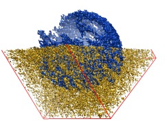
Place spherical markers | (June 18, 2010, version 1.4, details, video) |
Spherical markers can be hand placed in a density map, for example, to show the position and size of vesicles in electron microscopy. The markers are place using the mouse and settings in the Volume Tracer dialog.
Tools / Volume Data / Volume Tracer
Markers can be hand-placed on data with low signal-to-noise by viewing a single data plane and clicking to create a spherical marker and dragging to move or resize the marker. The useful settings in for this in the Mouse menu of the Volume Tracer dialog are
Place markers on surfaces [on]
Move and resize markers [on]
Place markers on high density [off]
Link new marker to selected marker [off]
Also it is convenient to use button 3 (the right mouse button) if you have a 3-button mouse with a scroll-wheel since the normal button 3 zooming action can be done with the scroll wheel.
Clicking on the displayed density will place a marker. Its color and radius can be set with fields in the Volume Tracer dialog. It can be moved by clicking on it and dragging. Holding the shift key will allow moving it in the direction perpendicular to the screen. Engaging the caps-lock key allows adjusting the marker radius by clicking on it and dragging up or down.
The default volume tracer mouse mode settings are more suitable for placing markers on data with better signal-to-noise such as single-particle EM reconstructions. This use is described here.
Find symmetry axis | (January 2009, version 1.4, details) |
A symmetry axis of a map can be located using the measure rotation command. The basic procedure is to make a copy of the map, rotate it by hand to a symmetrical position, optimize that alignment, then measure the axis of rotation between the original map and the copy. To make the map copy use volume dialog menu entry
File / Duplicate
Then rotate the map copy by hand about the observed symmetry and optimize its fit in the original map using the Fit in Map dialog. To determine the symmetry axis accurately it helps to rotate by an angle near 180 degrees, for example, for 7-fold symmetry rotate 3/7 or 4/7 of a full turn. To calculate the axis use a command like
measure rotation #0 #1 color orange
where the two maps have id numbers 0 and 1. The axis will be displayed as a rod that is defined as two spherical markers joined by a cylinder (equivalent to two atoms and a bond). The axis is a new model with its own id number shown in the Model Panel dialog (menu Favorites / Model Panel). The map copy can be deleted. To rotate a map or any Chimera model about this axis use a command like
turn #2 45 models #1
where the model id of the axis is 2, the rotated model has id 1, and the rotation is by 45 degrees. You can quantify approximate symmetries by plotting the correlation of a map with a rotated copy of itself using command measure correlation.
IMOD surfaces | (October 2007, version 1.2454, details) |
Surfaces enclosing structures in tomography data created in the IMOD software package can be displayed in Chimera. Simply open the IMOD binary files with file suffix .imod or .mod using Chimera menu entry
File / Open....
The surfaces are created in IMOD by drawing contours, loops or curves, plane by plane within the map data which are then connected into surfaces. The file must contain mesh data which can be created from the contour data with the imodmesh program.
Individual imod objects can be selected with the mouse. Some Chimera keyboard shortcuts (enabled with menu entry Tools / General Controls / Accelerators On) are helpful for manipulating these selected objects:
Placing the mouse over a surface will show the IMOD name for that object in a pop-up balloon. A map can be masked to within the selected surfaces using the mask command. The surfaces can be colored according to map density using the Surface Color tool.
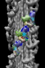
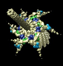
Symmetric fitting | (October 2007, version 1.2456, details) |
When fitting an atomic model into a map with symmetry, copies of the atomic model can be automatically placed to preserve symmetry as the original copy is fit. This helps see steric clashes between neighboring copies of the atomic model as the fitting is performed. Use the command "sym" to create the multiple symmetry-tracking copies of an atomic model. This command is typed to the Chimera command line at the bottom of the main Chimera window. To display the Chimera command line use menu entry
Favorites / Command Line
The command uses matrices specified in the PDB file header to position the symmetric copies. These usually have to be added in a text editor. Each 3 row and 4 column matrix gives a 3 by 3 rotation matrix in the first 3 columns and a following translation in the last column. These transforms are applied relative to the map coordinate system. Here is an example for the helical symmetry shown in the above myosin image:
REMARK 350   BIOMT1   1  1 0 0 0
REMARK 350   BIOMT2   1  0 1 0 0
REMARK 350   BIOMT3   1  0 0 1 0
REMARK 350   BIOMT1   5  0.866025 -0.5 0 0
REMARK 350   BIOMT2   5  0.5 0.866025 0 0
REMARK 350   BIOMT3   5  0 0 1 145
REMARK 350   BIOMT1   9  0.866025 0.5 0 0
REMARK 350   BIOMT2   9  -0.5 0.866025 0 0
REMARK 350   BIOMT3   9  0 0 1 -145
If you have multiple PDB models or multiple maps open you can specify the id numbers of the desired PDB model and map in the sym command. For example,
sym #1 #0
would use PDB model with id number 1 and map with id number 0. Use menu entry Favorites / Model Panel to see the id numbers of the open data sets. The ~sym command removes the symmetric copies.
Fit map in map | (November 2006, version 1.2315, details) |
One density map can be fit within another. The first map is hand-placed using the mouse into the second map, and then a local optimization of the overlap between maps can be performed. To move one map with the other held fixed use menu entry
Favorites / Model Panel
Switch off the checkbutton in the first column (heading Active) of the Model Panel dialog next to the map that will be frozen. Now move the other map with the mouse (buttons 1 and 2) to an approximately correct position in the frozen map.
To locally optimize the position of the map use menu entry
Tools / Volume Data / Fit Map in Map
This tool moves and orients the map to maximize the overlap (sum of pointwise products of map values). It uses a steepest ascent algorithm and only finds the locally optimal position. Select the two maps and press the Fit button. The map is moved to the locally optimal position after up to 100 steps. The correlation between the two maps is reported.
Note that the overlap is optimized, not the correlation. The correlation is just the overlap normalized by the sum of squares of the map values. Because the correlation is calculated only using points within the displayed contour level of the map being placed, the normalization factor for the second map varies according to fit position. So optimizing overlap is not equivalent to optimizing correlation. A noticable consequence is that the fit map will be pushed towards higher density regions even if the pattern of density variation does not match.
Fit model in map | (November 2005, version 1.2186, details) |
Atomic models can be fit into a density map by hand with the mouse and a local optimization of the fit position can be performed. To move an atomic model while keeping a density map fixed use
Favorites / Model Panel
Switch off the checkbutton in the first column (heading Active) of the Model Panel dialog next to the name of the density map. This locks the map position. Now move the atomic model with the mouse (buttons 1 and 2) to an approximately correct position in the map.
To locally optimize the position of the model in the map use menu entry
Tools / Volume Data / Fit Model in Map
This tool moves and orients the model to maximize the sum of density values at selected atom positions. It uses a steepest ascent algorithm and only finds locally optimal positions. Select atoms of the model to use in the fit (for example, menu entry Select / All) and press the Fit button. The model is moved and the average density value and the size of the motion (translation and rotation) are reported in the reply log (menu entry Favorites / Reply log).
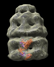
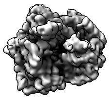
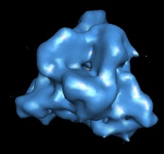
The map shown is of E. coli chaperonin (EM database entry 1046) and the fit model is PDB 1grl.
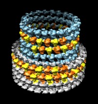
Place markers | (August 2005, version 1.2154, details) |
|
| 
| 
|
| Zone near markers | Color near markers |
Markers can be placed on volume data with the mouse. Use menu entry
Tools / Volume Data / Volume Tracer.
Then hold the ctrl key and click with the third mouse button (rightmost) on the volume surface to drop a marker. A marker will be placed on the first maximum of the volume data along the line of sight under the mouse position. The marker appears as a sphere. Links are drawn between consecutively placed markers. Markers and links can be given different colors and radii or can be deleted. Click the Markers button at the top of the volume tracer dialog to expand the dialog to show these additional controls.
Markers can be used for restricting volume data display to a region near the markers (see zone display), or to color the volume surface near the markers (see zone coloring), or their positions can be written to a file (click the volume tracer dialog Sets button and use Export XML).
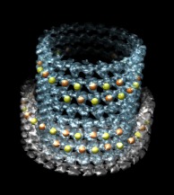
The image shows a segment of a two layer tubulin fiber. Alpha and beta tubulin proteins have different colored markers. (EM database entries: inner layer 1129, outer layer 1130). The maps have opposite handedness as those shown in the publication Nature. 2005 Jun 16;435(7044):911-5. This is most likely an error in the deposited data files.
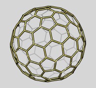
Icosahedral cage | (October 2007, version 1.2466, details hkcage and meshmol) |
An icosahedral reference lattice can be shown for comparison to virus capsids, clathrin cages, carboxysomes and other icosahedral structures. This uses the hkcage command:
hkcage 2 1 linewidth 3 color blue sphere 0.8
The integer parameters h=2 and k=1 describing the arrangement of hexagons and pentagons are described in the hkcage documentation. The cage can have flat triangular facets (sphere 0.0) or be spherical (sphere 1.0) or any radially interpolated intermediate.
The cage is a surface model shown as a mesh. The mesh lines are two dimensional. To make the cage lines cylinders you can make convert the surface model into a molecular model with the meshmol command which takes the model number and the cylinder radius as parameters.
meshmol #0 2.5
The resulting model can be saved as a PDB file with File / Save PDB....
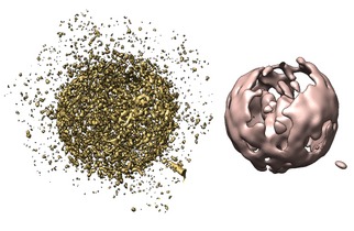
Local correlation | (October 2012, version 1.7, details, video) |
The vop localcorr measures the local correlation between two maps using a moving window of size N by N by N grid points (default N = 5). It can be used to see where two aligned maps are similar and where they differ. To compare two maps use
vop localCorrelation #0 #1
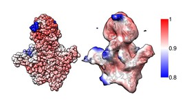
which will produce a new map containing correlation values (-1 to 1) where the correlation at each grid point is computed over a box centered at that grid point of N by N by N grid points. This new map can be used to color one of the original maps using the Surface Color dialog or with the equivalent command
scolor #0 volume #2 cmap 0.8,red:0.9,white:1,blue
To find the local correlation of a molecular model with a map the molmap command can be used to make a simulated map for a molecular model. Then the Values at Atom Postions dialog combined with the Render by Attribute dialog can be used to color atoms according to the local correlation at the atom positions.
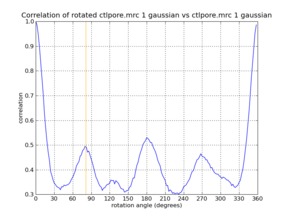
Degree of symmetry | (January 2009, version 1.4, details) |
The measure correlation command can be used to assess approximate symmetry of a map by plotting correlation of the map with a copy of itself rotated about the symmetry axis as a function of rotation angle. The command looks like:
measure corr #1 #0 rot #2
where the map, its copy, and the rotation axis have model id numbers 0, 1 and 2. To create the symmetry axis and a copy of the map refer to the find symmetry axis description. The command creates a plot in a separate window showing correlation coefficient versus rotation angle. Clicking and dragging in the plot window will rotate the map copy to the corresponding angle and show an vertical line at that position in the plot window. The plot image can be saved.
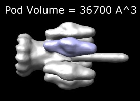
Measure volume | (November 2005, version 1.2186, details) |
The volume enclosed by a surface can be measured. This can be used for estimating the size of proteins that would occupy that volume. Use menu entry
Tools / Volume Data / Measure Volume.
Select a surface using the menu in the measure volume dialog and press the Compute Volume button. If the surface has several disconnected components, the computed volume is the sum of the volumes of all components. To measure the volume of just one component you can use volume subregion selection or volume erasing to get a surface of just the desired part. If the surface has any holes then no volume will be computed. For a contour surface, holes will only be present if the high density region hits the edge of the data set box. In this case zeroing the boundary of the data set will close the holes.
The image shows the phage p22 tail, EM database entry 1119. Subregion selection was used to cut out one of the 6 pods (purple). The boundary of that subregion was zeroed to close a hole where it connects to the tail body. The volume was displayed in the image using the Chimera 2D Label utility (menu entry Tools / Utilities / 2D Labels).
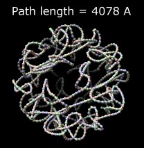
Path length | (November 2005, version 1.2186, details) |
The length of a path created with the volume tracer can be measured. This is done with keyboard accelerator pl. Keyboard accelerators are turned off by default. To activate them use menu entry
Tools / General Controls / Accelerators On
Then select the path (for example, by dragging a box around it with ctrl button 1) and type pl in the graphics window. The path length is reported at the bottom of the main window status line and also is reported in the Reply Log (shown with menu entry Favorites / Reply Log). The path length accelerator works on any set of selected bonds. They need not form a single chain.
The image shows a model of the 1056 nucleotide single stranded RNA genome of satellite tobacco mosaic virus. The path length was displayed in the image using the Chimera 2D Label utility (menu entry Tools / Utilities / 2D Labels).
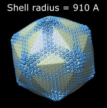
Shell radius | (November 2005, version 1.2186, details) |
The radius of a spherical or icosahedral shell can be measured. This can be used for measuring layers of virus particles. Display the Icosahedron Surface tool with menu entry
Tools / Higher-Order Structure / Icosahedron Surface
The dialog can display a surface linearly interpolated between an icosahedron and a sphere. Use the Show button on the icosahedron surface tool to create the surface. The radius of the surface can be adjusted with the radius slider. With solid display style make the surface transparent by pressing the color button. On the color dialog press the Opacity button, and then adjust the slider labelled A, 0 = completely transparent, 1 = completely opaque.
To get a spherical shape or when interpolating between a sphere and an icosahedron, set the subdivision factor to a larger value, for example, 64. This is needed to produce the rounded shape. The sphere factor controls linear interpolation between icosahedron and sphere shapes, 0 = icosahedron, 1 = sphere.
If the density map is not centered at the origin (where the icosahedron is centered) then you can recenter it as described in the icosahedral slice example.
The image shows Paramecium Bursaria Chlorella Virus (PDB 1m4x) displayed using the Multiscale tool and a shell of radius 910 angstroms, with sphere factor = 0.42. The radius text on the image was added using the Chimera 2D Label utility (menu entry Tools / Utilities / 2D Labels).
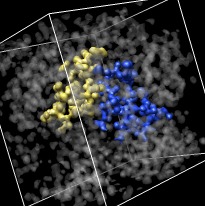
Color connected surface | (October 2007, version 1.2456, details) |
Connected surface components can be colored and there volume and area measured using menu entry
Tools / Volume Data / Pick Surface Pieces
The pick surface pieces dialog allows you to choose a mouse button (default ctrl-button-3) and color. Clicking on a surface colors the entire connected surface component under the mouse and reports its volume and area in the status line and reply log (Favorites / Reply Log). If the level of a volume contour surface is changed, all coloring done with this tool is lost. There is currently no way to save the coloring.
The example shows a unit cell of x-ray density for PDB model 1a0m. Two monomers have density not connected to any surrounding density at a contour level of one standard deviation and have been colored yellow and blue with volumes reported as 238 and 240 ų.
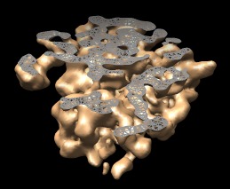
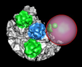
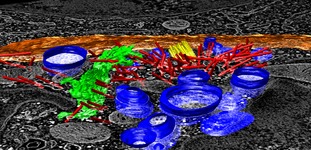
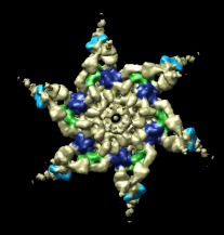
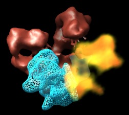
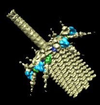
Color zone | (August 2005, version 1.2154, details) |
|
| 
| 
|
| Side view | Oblique view |
Patches of a surface near selected atoms or markers can be colored to match the atom or marker colors. Use menu entry
Tools / Volume Data / Color Zone
to show the color zone dialog. Select the atoms from a molecular structure or markers placed with the volume tracer tool by holding the ctrl key and clicking on them with the left mouse button, or dragging a box around them. Press the Color button on the color zone dialog to color portions of the surface within the specified distance.
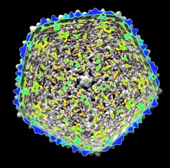
The image shows part of the phage T4 tail assembly. Regions of the EM density map near three structural proteins GP8, GP9, and GP11 are colored blue, green and cyan. (EM database entry 1089, and PDB model 1tja.)
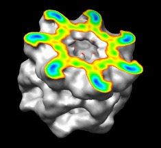
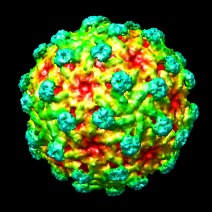
Radial coloring | (August 2005, version 1.2154, details) |
|
| 
|
| Higher contour level |
Surfaces can be colored according to radial distance. Use menu entry
Tools / Volume Data / Surface Color
to show the surface color dialog. Choose from the menu Using electrostatic potential, or other volume data, or by distance to color by Radius. To use radii ranging from the minimum to maximum radius for the surface press the Set full range colormap values button, then press the Color button at the bottom of the dialog to color the surface. The colors and radii can be changed and pressing the Color button again will update the coloring. The Origin entry field specifies where the radius is measured from.
The image shows a fibered phi29 virus particle colored red near the center and blue near the extremities. (EM database entry 1116.)
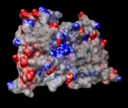
Electrostatic potential | (August 2005, version 1.2154, details) |
The image shows a solvent excluded molecular surface colored according to electrostatic potential. Blue represents positive potential and red negative. Zero potential is white, partially transparent. Chimera does not compute electrostatic potential, but can display electrostatic potential grid data computed by other programs (eg. DelPhi, APBS, UHBD).
To color a molecular surface open the molecular model (PDB 2sod in this image) and use menu entry
Actions / Surface / show
display the molecular surface. Use menu entry
Tools / Surface+Binding Analysis / Electrostatic Surface Coloring.
Click the Browse... button on the dialog that pops up and select the electrostatic grid file (sod.phi for this image). Then press the Color button.
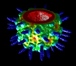
Color by density value | (August 2005, version 1.2154, details) |
A clipped and capped surface can be colored according to density map values using
Tools / Volume Data / Surface Color
A surface coloring dialog is shown. Press the Set full range colormap values button to fill in density values for a rainbow coloring spanning the range of density values found on the surface. Turn on the Only color sliced surface face switch if desired, and then press Color. The coloring will update whenever the clip plane position or surfacing threshold changes.
A map of GroEL is shown, sliced perpendicular to the cylinder axis (EM database entry 1080). Red is low density and blue is high density.
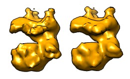
Morph map | (October 2007, version 1.2456, details) |
To linearly pointwise interpolate from one map to another use the morph map tool, menu entry
Tools / Volume Data / Morph Map
Choose the two maps and then move the Fraction slider to linearly interpolate between them, 0 corresponding to the first map, and 1 correpsonding to the second map. The interpolated map is shown in the volume dialog and the graphics window with settings initially matching those of the first map. Threshold levels and colors for the interpolated map can be changed in the volume dialog. The Play button gradually increases the interpolation factor to show a smooth animation between maps. The Record button can record this to a movie file.
This tool makes the differences between related maps visually evident but is not a reliable guide to how the structures undergo conformational changes. The example shows morphing between two RNA polymerase II conformations (EMDB 1283 and 1284).
Ambient Occlusion Lighting | (October 2007, version 1.2454, gaussian and surface color details) |
Contour surfaces with recesses can be made to look more 3-dimensional by darkening the recessed areas. If light cannot reach a deep pocket it should appear dark. The most direct way to achieve this is to shine lights on the surface from many directions and compute shadows. Chimera only has two lights and does not currently compute shadows. In some cases the same effect can be achieved using the Surface Color and Gaussian Filter tools as follows.
Use the Gaussian Filter tool, menu entry,
Tools / Volume Data / Gaussian Filter
to make a smoothed copy of the volume. Choose a Gaussian width about equal to the size of the recesses in the structure so the smoothed version is a featureless blob. Then use the Surface Color tool
Tools / Volume Data / Surface Color
to color the original volume using the smoothed volume values. Choose two colors, press the Set full range colormap values button, make the color with lower value light (e.g. white) and higher value dark (e.g. black). Then press the Color button. The smaller values in the Gaussian smoothed map are the outer parts of the original map while the larger values will be in recesses. Adjust the lower and upper data values and press the Color button to achieve the desired degree of shading.
The image shown is a Trypanosoma 80S ribosome (EMDB 1303). Silhouette edges (menu entry Tools / Viewing Controls / Effects) and reduced shininess (menu entry Tools / Viewing Controls / Shininess) have been used to increase the ambient occlusion depth effect.
Box face capping | (October 2007, version 1.2455, details) |
When a contour surface reaches the edge of the volume box the data values on the box faces that are higher than the contour level are covered with a flat surface coincident with the box face. These patches are not strictly contour surfaces since they pass through data values higher than the contour level.
This box face capping option is enabled by default and makes the contour surface appear solid having no holes. To turn off the face capping use volume dialog menu entry:
Features / Surface and Mesh Options
and switch off
Cap high values at box faces
Box face capping is usually preferable to placing zeros on the boundary of the data set because it gives perfectly flat surfaces, and works when showing different subregions of a volume data set.
Square mesh | (May 2006, version 1.2238, details) |
The default volume mesh display style shows a triangular mesh. To show just the contour lines in the xy, yz and xz grid planes use volume dialog menu entry
Features / Surface and Mesh Options
And turn on the Square mesh option. The mesh is then less opaque and the square mesh grid shows the grid plane spacing. Using a transparent mesh color is also helpful for seeing atomic models fit into a density map. You can make square meshes the default for future Chimera sessions using volume dialog menu entry
Features / Save default dialog settings
You probably want to close the surface and mesh options panel before saving the default settings since the currently displayed panels are also saved as the defaults.
Close boundary holes | (November 2005, version 1.2186, details) |
|
| 
| 
|
| Boundary zero. | Holes, unlit interior. | Holes, lit interior. |
When high density extends to the boundary a data set the contour surface shows a hole, and the inside of the surface is visible. Setting the map values on the boundary of the data set to zero eliminates the holes. This is done with keyboard accelerator zb. Keyboard accelerators are turned off by default. To activate them use menu entry
Tools / General Controls / Accelerators On
Then type zb in the graphics window to zero the volume data values on the 6 faces of the data set currently shown in the volume viewer dialog. A new writable copy of the data is created which can be saved to a new file using the volume viewer dialog menu entry File / Save Map As....
Closing the boundary holes is needed when computing the volume enclosed by surfaces, and to make capping of surfaces cut with clip planes work. It is also desirable to avoid visually confusing views of the interior of the surface. An alternative to improve appearance is to make the inside of the surface dark by turning off the Two-sided surface lighting option in the volume viewer dialog (menu entry Features / Surface and Mesh options).
The images show Paramecium Bursaria Chlorella Virus (PBCV-1) from the VIPERdb web site.
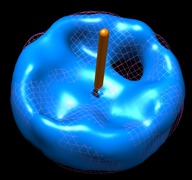
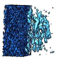
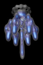
Smoothing surfaces | (August 2005, version 1.2154, details) |
The level of detail can be controlled by changing the Step setting near the top of the volume viewer dialog (menu entry Tools / Volume Data / Volume Viewer). A step setting of 2 2 2 means every other plane is used along the x, y and z axes of the data. A step of 1 1 1 uses all the data and shows the most detail.
You can additionally smooth the surface. This keeps the level of detail the same but reduces sharp edges and faceted appearance of the surface. This is in the Options panel of the volume viewer dialog. Check the Options button at the top of the dialog to expand a long list of options. At the bottom of the list turn on Surface smoothing iterations. This moves each vertex of the surface (which is made up of many triangles) towards the average position of adjoining vertices. Two parameters control the degree of smoothing. The fraction of the distance to move a vertex towards the average is one parameter, and the other is the number of times to repeat the smoothing.
The image shows a machine that regulates fusion of vesicles with membranes, N-ethyl maleimide sensitive factor (NSF). (EM database entry 1059). It has been colored by cylinder radius using the Surface Color tool. Two copies of the data set are shown with step 1 1 1 on the left and step 4 4 4 on the right, and smoothing turned on for both.
Multiple contour levels | (August 2005, version 1.2154, details) |
More than one contour level can be displayed. In the volume dialog (menu entry Tools / Volume Data / Volume Viewer) hold the ctrl key and click on the histogram to add a contour level. To see the nested surfaces color them distinctly and use transparency or mesh display style. To color a level, click its vertical bar on the histogram and then click on the square color button below the histogram. This shows the Color dialog. Press the Opacity button on the color dialog shows an additional slider labeled A that makes it possible to see through the surface.
The image shows 3 contour levels of the tail assembly of phage P22. (EM database entry 1119.)
Display styles | (August 2005, version 1.2154, details) |
Volume data can be displayed in 3 styles: contour surfaces, meshes, or solid style. There are checkbuttons on the volume dialog for the 3 styles. Mesh and surface are the same except that mesh just shows the edges of the triangles composing the surface. Solid style assigns a degree of transparency to every grid point in the volume and then displays the full semi-translucent data.
The image shows a potassium channel (EM database entry 1094) with half the tetramer as a red surface, a quarter as a blue mesh, and a quarter as a yellow solid rendering. To display the 3 different styles at the same time I opened 3 copies of the data and cropped each to show just part of the channel.