
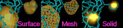
Volume Viewer is an tool for visualizing three-dimensional (3D) numerical data sets. Data can be shown as solid or mesh isosurfaces (contour surfaces) or as partially transparent solids. Some examples:
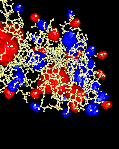
electrostatic potential (surfaces) |
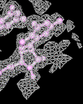
electron density map (mesh) |
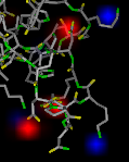
electrostatic potential (solids) |
The state of Volume Viewer is included in saved sessions. Volume Viewer is sometimes used together with Volume Path Tracer, which allows markers to be placed within volume data and connected by smooth, interpolated paths.
Volume Viewer is under development. New features are being added, and some limitations will be addressed in future versions.
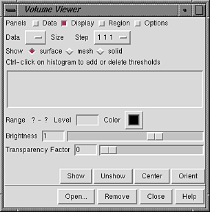
There are several ways to start Volume Viewer, a tool in the DelPhi, Docking, and Volumes categories. Starting Volume Viewer opens a panel.
| Volume Viewer Panel - initial appearance |
|---|
 |
| Format | Suffix | Description |
|---|---|---|
| APBS potential | .dx | electrostatic potential calculated with Adaptive Poisson-Boltzmann Solver (APBS) |
| BRIX or DSN6 | .brix .omap |
crystallographic density map used by O |
| CCP4 or MRC | .ccp4 .mrc |
crystallographic or EM density map |
| CNS or XPLOR | .cns .xplor |
unformatted ASCII density map |
| DelPhi or GRASP | .phi | electrostatic potential calculated with DelPhi (the academic version; see also DelPhiController) or GRASP |
| DOCK scoring grid | .bmp .cnt .nrg |
DOCK 4 bump, contact, and energy scoring grids (not interchangeable; gridname.bmp required for reading gridname.cnt and/or gridname.nrg) |
| NetCDF | .nc | generic portable array format |
| Priism | .xyzw | 3D light and electron microscope data |
| SPIDER | .spi | electron microscope density map |
| TOM toolbox EM density map | .em | electron microscope density map |
One of these types can be chosen from the File type: pulldown menu near the bottom of the dialog, or the type can be inferred from the suffix(es) of the chosen file(s). Additional file types can be defined. If a file is not in the correct format, an error message will usually appear.
By default, the data will be displayed automatically if it does not exceed a certain size (see Show data when opened... in the Options panel); data exceeding the size limit will not be displayed until the Show button near the bottom of the panel is clicked. It may be useful to adjust various parameters within the panel before clicking Show, however. More than one file can be opened, and more than one subregion or subsample from the same or different files can be displayed.
The data set information and display values shown in various sections of
the Volume Viewer Panel always refer to the currently selected data set
(or current set).
The current set is indicated next to the word Data
on the second line of the Volume Viewer Panel.
The current volume display
may correspond to part or all of the
current set of data.
VOLUME VIEWER PANEL ORGANIZATION
The Volume Viewer Panel has four subpanels, listed at the top next to checkboxes:
Clicking the adjacent checkbox expands the panel to show the corresponding section. Initially, the Display panel is shown and the others are hidden.| Volume Viewer Panel - basic components |
|---|
The current set is indicated next to the word Data on the second line of the Volume Viewer Panel. This is a pulldown menu when more than one data set is open, and a different set can be selected (made the current set) by choosing it from this menu or by clicking its entry in the Data Sets list in the Data panel. The Size is the number of data points spanning each dimension of the current volume display, and the Step values indicate the density of sampling. For example, 1 1 1 means all the data points are used to generate the display; 2 2 2 means every other data point is taken along each axis, reducing the number of data points used by a factor of eight. Changing step sizes with the pulldown Step menu turns off their automatic adjustment ( Adjust step to show at most [n] Mvoxels in the Options panel).
Show generates the current volume display from the current set of data according to the boundary settings in the Region panel and the color and rendering settings in the Display panel. Unshow deletes all (one or more) displays of the current set. The Center button scales and centers the view and adjusts the clipping planes to contain the current volume display. The Orient button reorients all open models so that the axes of the current set are pointing in the standard directions: X horizontal in the plane of the screen increasing rightward, Y vertical in the plane of the screen increasing upward, and Z perpendicular to the screen increasing outward from the screen.
Open... is used to open data files. Remove deletes the current set and its display(s). Help brings up this manual page in a browser window, and Close dismisses the Volume Viewer Panel. If the panel is closed accidentally, it can be reopened in the same state by reinvoking Volume Viewer.
The default settings will often suffice for displaying the data without performance problems. If there are problems, however, the first issue to address is the size of the data set: whether the information can be handled and displayed in a reasonable amount of time. Typically, an isosurface for a 64 x 64 x 64 data set can be displayed in a few seconds on a late-1990's machine. The Chimera web site includes a benchmark table listing the volume data sizes that can be handled at 10 frames per second on various computer systems. With the solid rendering mode, performance is optimal when region dimensions are powers of 2 (see the discussion on texture mapping). A status line near the bottom of the panel reports on the progress of a calculation. Some experimentation may be required to balance appearance and performance for a given data set. The size of a 3D data set is essentially the total number of values, X x Y x Z. It is related to both the physical dimensions (for example, angstroms along each axis) and the resolution (spacing) between data points. To decrease size, one can focus on a smaller physical region and/or use a sparser grid of points from the original data set. This can be done using the Region panel:
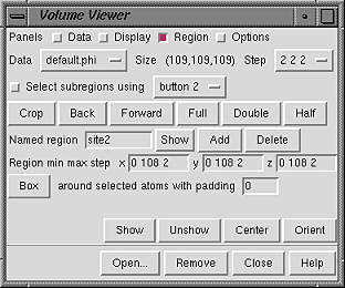 |
Select subregions using [button] allows subregions of the current set to be defined with the mouse. The indicated mouse button (which can be changed using the pulldown menu) is reassigned from its existing function to volume selection in the graphics window. A volume selection can only be a rectilinear box with axes corresponding to the original X,Y,Z axes of the current set. Depending on the viewing direction, this may be a surprisingly large box. It is often helpful to Orient the volume before defining a subregion.
In the following description of selection boxes, "clicking" and "dragging" refer to operations with whichever mouse button has been assigned to subregion selection. When there is no pre-existing selection box:
Half and Double change the physical extents of the current volume display by a factor of 2; Half halves the size in each dimension and Double doubles the size in each dimension, keeping the center the same. After a certain amount of zooming out, the min and max values shown may be beyond the bounds of the original data set, but the actual region displayed will be no larger than the original data. After one or more cycles of zooming in and out, the extents may differ from the original due to rounding. Full restores the original extents.
After various subregions of the current set have been used during a session to define the current volume display, it is possible to go Back and Forward among them. The subregion farthest Back is the earliest created within the session. Up to 32 subregions can be stored and traversed. Only changes in min and max values (not step sizes) are reflected in this history.
Subregions can also be named and then restored by name. The Named region line is shown only when Show named regions in region panel in the Options panel is turned on. In this line, Add adds the name entered in the name field to the list of named regions, Delete deletes the region with the name shown in the name field from the list of named regions, and Show allows restoration (from a pulldown menu) of any of the named regions on the list. When Add is clicked, the min and max values of the current volume display (not the volume selection box) are saved. A named region can also be restored by typing its name in the Named region field and pressing Enter (return).
The Region min, max, and step values are shown only when Show bounds and step in region panel in the Options panel is turned on. In the figure, there are 109 data points in each dimension, with grid indices running from 0 to 108. The step values are 2, meaning that only every other grid point in each dimension is used to calculate the display. This does not affect the physical extents of the displayed data. The physical extents can be decreased by increasing the min grid indices and/or decreasing the max grid indices. Because they refer to grid indices, the min, max, and step values must be integers. They can be changed manually by typing in new values and then clicking Show or pressing Enter (return). This updates the current volume display based on the new min, max, and step values and turns off automatic step size adjustment ( Adjust step to show at most [n] Mvoxels in the Options panel). The original full data set can be restored by changing the min, max, and step values back to their original settings (or clicking Full).
Another way to pare down the data set is to make an atom selection within a molecule or molecules shown in the graphics window, and then click the Box around selected atoms... button (only shown when Show atom box button in region panel in the Options panel is turned on). This sets the physical extents of the current volume display to a box with X,Y,Z dimensions enclosing the selected atoms. If some additional space around the atoms is needed, the desired increase in box size in every direction (in the current display units) can be typed into the padding field.
The Data panel includes a listing of open Data Sets:
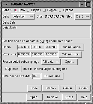 |
The X, Y, and Z Origin coordinates and Voxel size are shown for the current set. The Origin is the data point with indices (0,0,0), and Voxel size refers to the data point spacing (resolution). The values can be edited; changes take effect when the Enter (return) key is pressed. The position of the origin and the voxel dimensions can be restored to their starting values with Original origin and Original size, respectively.
Precomputed subsamplings are especially useful when the data set is large and when facile switching between viewing large subregions at low resolution and viewing smaller subregions at high resolution is needed. Precomputed subsample files decrease memory usage and time spent reading data. When a file is opened and listed as a Data Set, its contents are not read into memory until Show is pressed; thus, even when the full extents of the current set are being displayed, only a smaller precomputed subsample matching the Step values shown (if available) will actually occupy memory. Subsamples of the original data can be created with the program downsize.py. Besides the more efficient use of memory, another reason to use precomputed subsamplings instead of generating them on the fly is that downsize.py offers a variety of methods for determining the subsample values. The subsample files must be associated with the correct full data file when they are opened. This is done by opening the full data file, making sure it is the current set, and then using the Open... button in the Precomputed subsamplings to open the subsample files. Along with the full data, the subsamples are listed in the pulldown Precomputed subsamplings menu according to the Step sizes inferred to have been used to generate them from the full data file. When Show is pressed, the appropriate subsample (based on Step values) is used.
It is also possible to open and work with precomputed subsample files in the "normal" way (without associating them with the full data file). However, this does not allow for easy switching among different subsamplings of the same full data set.
Duplicate makes a copy of the current set so that opening the same file multiple times is not required for simultaneously displaying different subregions or different representations of the data.
The Data cache size setting controls whether volume data is kept in memory when it is not being displayed. A cache can improve performance, since accessing data in the cache is faster than reading it from disk. It is necessary to press Enter (return) after changing the cache size. Undisplayed data is purged from the cache to maintain the size, but if the displayed data alone requires more space, it will not be purged. The least recently displayed data is purged. The data cache only accounts for part of the memory used by Volume Viewer. Because a significant amount of additional memory is occupied by surfaces and color arrays used in rendering, the cache size should be set to about 1/3 or 1/2 of the desired total memory usage by Volume Viewer. Clicking Current use opens a dialog showing how much memory is occupied by volume data (not including the surfaces, etc. mentioned above).
A Priism or NetCDF file can contain more than one 3D array of values (more than one component). Thus, each grid point can have several data values, for example corresponding to the different wavelengths used to image a specimen. Each component has its own threshold(s) and color(s). When multiple components (but not diffent subregions) of the same data set are rendered in the solid mode, their colors and transparencies are blended. The appearance of a solid display of multiple-component data may be suboptimal if a colormap is used (see the Options panel). A figure below shows the Volume Viewer Panel during solid display of three-component data.
 |
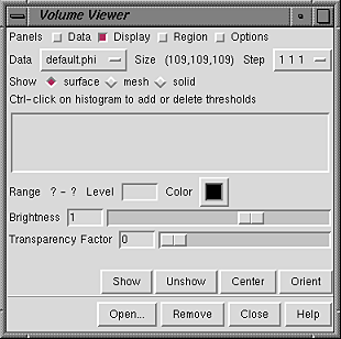
The rendering mode (surface, mesh, or solid) is indicated next to Show near the top of the Display panel. The surface and mesh modes depict isosurfaces (contour surfaces) consisting of a large collection of triangles. In the surface mode, each triangle is drawn as a plane of color. In the mesh mode, just the triangle edges are displayed. In the solid mode, the data is shown as a semitransparent solid. There are several rendering options.
Surface and mesh displays are of class Surface_Model. A solid display is of class Volume_Model. Each is opened as the lowest available model number and positioned in the same coordinate system as the otherwise lowest-ID-number model currently shown. Various buttons on the Volume Viewer Panel and/or the Model Panel can be used to control volume display models.
Rendering mode, thresholds, and colors are controlled in the Display panel. No histogram or threshold is shown until the data is displayed, either automatically upon opening if the data does not exceed a certain size (see Show data when opened... in the Options panel) or after Show is pressed.
| Volume Viewer Panel - before data display |
|---|
 |
When the current set has multiple components, the display of an individual component can be toggled on and off by clicking its Hide checkbox (see the figure below).
SURFACE OR MESH DISPLAYFor the surface and mesh rendering modes, each threshold is shown as a vertical bar. The example shows single-component data (electrostatic potential) contoured in cyan at a negative value and in magenta at a positive value.
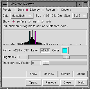 |
Any number of thresholds (contour levels) can be added by Ctrl-clicking with the left mouse button on the histogram. Ctrl-clicking on an existing threshold deletes it. Of course, different thresholds can have different settings for Level and Color; the settings shown apply to the threshold most recently moved or clicked, the current threshold. A threshold can be moved by changing the Level and then pressing Enter (return) or by dragging it horizontally with the left mouse button. Holding the Shift key down reduces the speed (mouse sensitivity) of threshold dragging tenfold, allowing finer control. Setting a contour level very low can generate a surface with many triangles that takes a long time to display.
Clicking the color well marked Color opens the Chimera Color Editor, in which a color for the display can be defined. Clicking the Opacity button on the Color Editor allows transparency to be included in the definition. However, since transparency can also be introduced with the Transparency Factor slider, it is not necessary to include transparency in the color definition to create a transparent display. Each threshold is shown in the same color as its display.
The Brightness slider scales the intensity of the color. A slider value of 1 produces no change relative to the intensities specified in the Color Editor.
The Transparency Factor ranges from 0 to 1 and is the fraction of light transmitted from behind the surface or a line of mesh.
When Dim transparent surface/mesh in the Options panel is turned on, brightness is automatically decreased when transparency is increased with the Transparency Factor slider or in the color definition (although this adjustment is not shown in the Brightness slider). There are also Options to control mesh line width and smoothing and the lighting of mesh and surface displays.
SOLID DISPLAYFor the solid rendering mode, each threshold is shown as a small square. The example shows three-component data (light microscope data at three wavelengths) with the components displayed in green, red, and blue.
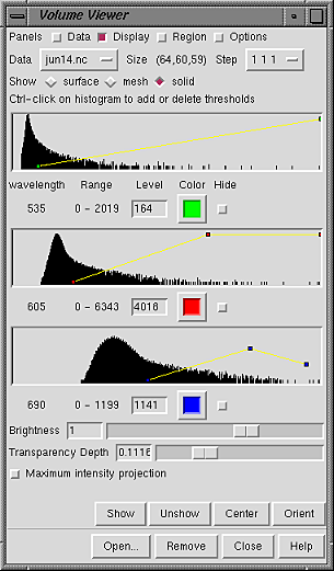 |
Any number of thresholds can be added by Ctrl-clicking with the left mouse button on the histogram. Ctrl-clicking on an existing threshold deletes it. Of course, different thresholds can have different settings for Level and Color; the settings shown apply to the threshold most recently moved or clicked, the current threshold. A threshold can be moved by changing the Level and then pressing Enter (return) or by dragging it horizontally and/or vertically with the left mouse button. Holding the Shift key down reduces the speed (mouse sensitivity) of threshold dragging tenfold, allowing finer control. The rightmost threshold does not have to be at the far right of the histogram, and a threshold at a lower data value can be higher (vertically) than a threshold at a higher data value.
Clicking the color well marked Color opens the Chimera Color Editor, in which a color for the display can be defined. Clicking the Opacity button on the Color Editor allows transparency to be included in the definition. However, transparency is inherent in the solid rendering mode, so it is not necessary to include transparency in the color definition to create a transparent solid display. Each threshold is shown in the same color as its display. Different thresholds for the same data component can be colored alike (as in the example) or differently.
The thresholds and connecting lines on each histogram define a function that maps data values to colors and intensities. For each voxel, the data value is compared to the thresholds on the histogram. The colors and intensities of the closest threshold at a lower data value (to the left) and the closest threshold at a higher data value (to the right) are linearly interpolated. Voxels with data values greater than the rightmost threshold or less than the leftmost threshold are colorless and completely transparent. Color is defined by red, green, blue and opacity components. The intensity at a threshold is further scaled by its vertical position, where 0 is the bottom of the histogram and 1 is the top. Rendering time does not depend on the positions of the thresholds, but increases with greater numbers of thresholds.
The Brightness slider scales the intensity of the color. A slider value of 1 produces no change relative to the intensities specified in the Color Editor.
The Transparency Depth is the thickness of a slab containing a color of full intensity (as for a threshold at the top of the histogram) that would block half the light from behind. Increasing the depth makes the volume more transparent and brighter, because less light is blocked. The Brightness slider can be used to compensate for this effect.
The Maximum intensity projection shows, at each pixel, the the most intense color value underlying the pixel (along the line of sight). The maximum intensities of the red, green, and blue color components are determined separately, after colors from multiple data components (if present) are blended. Transparency/opacity is not used; that is, the Transparency Depth and the vertical positions of the thresholds are ignored when this setting is on. The Maximum intensity projection can be useful for enhancing detail. Unphysical effects can result, but are usually not very noticeable; examples include the disappearance of a dim spot when it passes in front of a brighter spot and the simulation of a single spot when the maximal values of different color components under the same pixel actually come from different spots.
Several settings in the Options panel affect solid displays.
The default settings of the Options panel are shown in the figure:
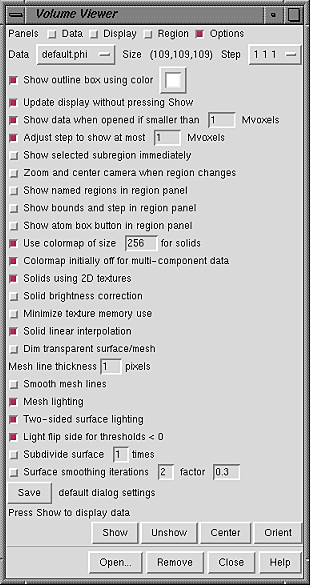 |
This option shows the bounding box of the current volume display. Clicking the color well opens the Chimera Color Editor, in which a color can be defined.
Update display without pressing ShowThis option causes automatic display updates upon changes in rendering mode, thresholds, colors, or Hide status in the Display panel or rendering settings in the Options panel. If this option is turned off, it is necessary to press Show to update the display after such changes. This option does not apply to display after:
This enables automatic initial display of data sets smaller than a specified size. The default limit of 1 Mvoxel (220 or 1,048,576 voxels) is equivalent to a 128 x 128 x 64 data set. The limit does not have to be an integer; for example, 0.25 could be used. When the option is on, a newly opened data set that exceeds the size limit will not be displayed until Show is clicked. When the option is off, Show must always be clicked to generate an initial display. Turning the option on or off or changing the Mvoxel limit will not affect the display of any data that has already been opened.
Adjust step to show at most [n] MvoxelsThis is a convenient way to limit the display to a reasonable amount of data. The default limit of 1 Mvoxel (220 or 1,048,576 voxels) is equivalent to a 128 x 128 x 64 data set. The limit does not have to be an integer; for example, 0.25 could be used. Note that the Step values are adjusted automatically by powers of 2 to comply with the Mvoxel limit (increased when the extents are increased, if necessary, and decreased when the overall region size is small enough for finer sampling). This option is turned off by:
This option automatically updates the display after selecting a subregion with the mouse (when the mouse button is released) but not after typing new min, max or step values in the Region panel. After such changes, it is still necessary to click Show or press Enter (return) to update the display.
Zoom and center camera when region changesThis automatically adjusts the view to fit the region when Show is clicked (and upon automatic display updates when Show selected subregion immediately is also turned on).
Show named regions in region panelWhether to include an interface to named regions in the Region panel.
Show bounds and step in region panelWhether to show min, max, and step values in the Region panel.
Show atom box button in region panelWhether to include the Box around selected atoms... option in the Region panel.
Use colormap of size [N] for solidsUsing a colormap allows faster, automatic updates of displays in the solid rendering mode when colors, thresholds, Brightness or Transparency Depth are adjusted. With some hardware, however, the updates may be too slow to be useful.
Data values for a region are divided into N ranges, with each range mapped to a particular color and transparency. N must be a positive integer. Smaller values of N result in coarser divisions and less smooth gradations of color. If N is set too high for the graphics hardware, an error message may result, or (depending on the GL implementation) the model may simply fail to appear. The hardware-determined maximum N is typically 256 or 65356.
Colormap initially off for multi-component dataA colormap allows faster updates of displays in the solid rendering mode but yields distinct colors rather than smoothly graded ranges. Noticeably abrupt color gradations are especially likely with multiple-component data, since the product of the numbers of divisions within the components cannot exceed N (specified with Use colormap...). For example, if N=256 and the data set has two components, there can only be 16 divisions for each component, such that any combination of the two values will map to one of the 256 color/transparency settings. Since the quality of display using a colormap may be low for multiple-component data, it is often best to check the performance without a colormap. If display updates are too slow without a colormap, Use colormap... can be activated.
Solids using 2D texturesThis switch controls whether the 2D or 3D texture mapping projection code is used for displays in the solid rendering mode. These give similar but not equivalent visual results. The 3D texture mapping method is not supported by some computer hardware. If 3D texture mapping is chosen but not supported by the computer hardware, an empty red outline box will be shown. If the hardware does support 3D texture mapping but the texture is too large, an empty yellow outline box will be shown. The 2D texture mapping method requires 3 times as much texture memory as the 3D method, but has the advantage of working on all platforms.
The region size that can be displayed may be limited by the amount of texture memory in the graphics card. Our late-1990's SGI systems are limited to 128 x 128 x 128 regions for 3D textures, but can handle larger regions with 2D textures. Regions requiring more memory than the graphics card has will work on some hardware, but with significantly degraded performance. The memory required is usually 4 bytes per volume element for the 3D texture implementation and 12 bytes per volume element for the 2D texture implementation. OpenGL restricts texture sizes to be powers of 2. If you try to display a 65 x 65 x 65 volume, the texture memory requirements and rendering speed will be like those for a 128 x 128 x 128 volume, since 128 is the smallest power of 2 that will accomodate 65 data values. Performance is optimal for regions with dimensions that are powers of 2.
Solid brightness correctionThis option only affects displays in the solid rendering mode with 2D texture mapping. If the brightness correction is turned off, the displayed brightness (and transparency) will depend on the viewing angle relative to the XYZ data axes. For a cube-shaped volume with equal resolution in the X, Y, and Z dimensions, the brightness drops and the transparency increases by a factor of sqrt(3) = 1.7 as the viewing angle is changed from along any axis to along the (1,1,1) direction (the cube diagonal). Turning on the brightness correction remedies this, but doubles rendering time.
Minimize texture memory useThis option only affects displays in the solid rendering mode with 2D texture mapping. Activating this option causes such displays to reuse a single 2D texture instead of allocating separate textures for every plane of the data volume. This is useful for viewing large data sets that would otherwise fail to display, but it can degrade performance (increase the lag time) when the display is rotated and during remote display.
Solid linear interpolationThis option only affects displays in the solid rendering mode. It causes linear interpolation of the brightness and transparency between voxels (in 2 dimensions for 2D texture mapping, all 3 dimensions for 3D texture mapping). Turning the option off may yield a pixelated look since the brightness and transparency across a voxel are constant, but may decrease the rendering time on some graphics hardware.
Dim transparent surface/meshThis option decreases the brightness of transparent volume models in the surface or mesh rendering mode as their transparency is increased. Specular highlights are also dimmed. Otherwise, increasing the transparency of a color (without changing its brightness) allows more light to shine through, resulting in an increase in the overall brightness. When dimming is on, OpenGL (alpha,1-alpha) blending is used instead of (1,1-alpha) blending.
Mesh line thickness [N] pixelsN is the pixel line width used in the mesh rendering mode; it must be a positive integer.
Smooth mesh linesDisplays in the mesh rendering mode consist of many lines. OpenGL can render smooth lines using anti-aliasing, but the method has a side effect: dense meshes look brighter from some viewpoints and darker from others, depending on the order in which the lines were drawn. Thus, anti-aliasing to smooth the lines is off by default, but can be turned on with this option. Only opaque mesh lines are affected; smoothing is always turned off for transparent lines because it is incompatible with the transparent rendering procedure.
Mesh lightingMesh lighting makes the inside of a contour volume shown in the mesh rendering mode dimmer than the outside. With mesh lighting on, the brightness varies according to the angle between each surface point normal and the line of sight; brightness is maximal when the outward-facing normal is parallel to the line of sight and pointing at the user (see more on the definition of "outward" under Light flip side...). With mesh lighting off, the brightness is uniform regardless of the angle between the normal and the line of sight.
Two-sided surface lightingTwo-sided surface lighting makes both the inside and outside of a contour volume shown in the surface rendering mode bright. Otherwise, only the outside is lit (see more on the definition of "outside" under Light flip side...). The brightness of each lit side varies according to the angle between a surface point normal and the line of sight; brightness is maximal when the normal is parallel to the line of sight.
Light flip side for thresholds < 0This option affects displays in the surface and mesh rendering modes. The surface mode is affected only when lit from a single side (when Two-sided surface lighting is off). The mesh mode is affected only when Mesh lighting is on. When Light flip side... is off, the side toward smaller or more negative data values is always treated as the outside of a contour volume. When Light flip side... is on, the side toward larger or more positive values is treated as the outside for any negative thresholds (contour levels), while the side toward smaller or more negative values is treated as the outside for any positive thresholds. Flip side lighting is appropriate when displaying data for which the sign is meaningful, such as electrostatic potential. In other cases, the data set is better described as a monotonic range of values, and where it lies relative to zero is not meaningful.
Subdivide surface [N] timesThis option increases the number of triangles used in the surface and mesh rendering modes. Subdivision can help to produce smoother surfaces when combined with the Surface smoothing... option. During a single round of subdivision, each triangle is divided into four smaller triangles by connecting the midpoints of the triangle edges. Thus, the number of triangles is increased by a factor of 4N, where N is a positive integer.
Surface smoothing iterations [N] factor [f]This option smooths displays in the surface and mesh rendering modes by moving each vertex toward the average position of its neighboring vertices (those connected by triangle edges). A vertex is moved a fraction f (ranging from 0 to 1) of the way toward the average position of its neighbors, and each vertex is moved once per iteration. N iterations are performed, where N is a positive integer. When Subdivide surface... is on, it may be necessary to use more smoothing iterations and/or a higher factor to achieve a smoothness similar to that of the unsubdivided surface.
Save default dialog settingsSave options and other settings as preferences.
Several preferences specific to Volume Viewer can be saved in the Chimera preferences file. Clicking Save default dialog settings in the Options panel saves all settings in that panel plus the data cache size from the Data panel and the subregion selection setting from the Region panel (whether subregion selection is turned on and which mouse button is assigned).
Several other settings tend to be specific to a particular volume data set and are not saved in this way. However, such settings can be saved along with an entire Chimera session in which Volume Viewer is being used (see SimpleSession).
The following standalone programs for converting, inspecting, and processing volume data files come with Chimera. They are found in the directory chimera/share/VolumeProcessing. The term "grid file" refers to any of the file formats read by Volume Viewer. All of the programs that produce a new volume write it in NetCDF format only.
The standalone programs use Python code that is provided with Chimera.
A current problem is that the location of these code files
must be indicated explicitly before the programs can run.
The PYTHONPATH environmental variable must be set
(adjust the examples as needed based on where Chimera is installed).
For example, on UNIX (in csh):
prompt> setenv PYTHONPATH /usr/local/chimera/lib:/usr/local/chimera/lib/Numeric:/usr/local/chimera/shareOn Windows, an analogous command is required:
prompt> PYTHONPATH=c:\Progra~1\Chimera\lib;c:\Progra~1\Chimera\lib\Numeric;c:\Progra~1\Chimera\share
| Program | Description |
|---|---|
| apply.py | Apply a function to a grid file pointwise. |
| combine.py | Add, subtract or multiply two grid files pointwise. |
| downsize.py | Reduce data size by subsampling. |
| gaussian.py | Convolve with a Gaussian of specified linewidth. |
| ridges.py | Create a derived volume revealing ridges and valleys. |
| showheader.py | Show the header of a grid file. |
| subregion.py | Extract a subregion from a grid file. |
| tonetcdf.py | Convert a grid file to NetCDF format. |
All of the programs take command-line arguments like input file names, numeric parameters, and output file names. The types of input files are recognized by the standard file suffixes. The standard suffixes are listed in the grid_formats.py file (the built-in formats and their suffixes are listed above). If the input file does not have the expected suffix, the file type can be specified on the command line by appending a colon followed by the file type (for example, mydata:delphi). Invoking any of the programs without arguments generates a short message describing the program and the needed command-line arguments.
Command-line UseTo use the programs on UNIX, add the directory to your search path. For csh (C shell), this looks like:
        % setenv PYTHONPATH /usr/local/chimera/lib:/usr/local/chimera/lib/Numeric:/usr/local/chimera/share
	% set path = (/usr/local/chimera/share/VolumeProcessing $path)
	% showheader.py 1a0m.omap
	Header for 1a0m.omap
	  size:                 92           98           88
	  xyz origin:    -1.734375    -9.365625   -5.5486111
	  xyz step:       0.346875     0.346875   0.32638889
	%
On Windows, use the DOS command prompt:
        > PYTHONPATH=c:\Progra~1\Chimera\lib;c:\Progra~1\Chimera\lib\Numeric;c:\Progra~1\Chimera\share
	> PATH=%PATH%;c:\Program Files\chimera\share\VolumeProcessing
	> showheader.py 1a0m.omap
	Header for 1a0m.omap
	  size:                 92           98           88
	  xyz origin:    -1.734375    -9.365625   -5.5486111
	  xyz step:       0.346875     0.346875   0.32638889
	>
Program apply.py
Apply a function to a grid pointwise. The resulting volume is written in NetCDF format.
Syntax: apply.py sqrt|square|abs|exp|log <infile> <outfile>Program combine.py
Add, subtract or multiply two grid data files pointwise and write the result as a NetCDF file.
Syntax: combine.py add|subtract|multiply <infile1> <infile2> <outfile>Program downsize.py
Reduce the size of a grid file by taking the average, maximum, minimum, or signed value of maximum magnitude over cells. The default mode is average. Produce a NetCDF output file. The cell sizes are equivalent to the Step sizes in the Region panel that would be used to generate the subsample on the fly. The output can be used as Precomputed subsamplings in the Data panel.
Syntax: downsize.py [-t ave|max|min|maxmag]
                    <x-cell-size> <y-cell-size> <z-cell-size>
                    <in-file> <netcdf-out-file>
Program gaussian.py
Convolve a Gaussian with grid file and write the result as a NetCDF file. The linewidth is specified in XYZ space units and spans -1 SD to +1 SD.
Syntax: gaussian.py <infile> <linewidth> <outfile>Program ridges.py
Count the neighbors of each volume element that have lesser value. The 26 neighbors in the 3 by 3 by 3 cube centered at an element are examined. The count is shifted by -13 so 0 represents an equal number of neighbors of greater and lesser value. The resulting volume is written in NetCDF format.
Syntax: ridges.py <infile> <outfile>Program showheader.py
Show grid size, XYZ origin and XYZ step. The XYZ origin and step are specified in the appropriate physical units for the data, e.g. angstroms, nanometers, microns. These coordinates are used when the data file is displayed in Chimera so that it aligns properly with model structures.
Syntax: showheader.py <filename> ...Program subregion.py
Write a subregion of a grid file in NetCDF format. The file written contains the data within and including the specified index bounds.
Syntax: subregion.py <infile>
                     <imin> <imax> <jmin> <jmax> <kmin> <kmax>
                     <netcdf-outfile>
Program tonetcdf.py
Write a grid file in NetCDF format. The position and scale of the matrix in XYZ coordinate space can be changed.
Syntax: tonetcdf.py <infile> <outfile>
                    [-origin <xorigin> <yorigin> <zorigin>]
                    [-step <xstep> <ystep> <zstep>]
A new file format can be added using Python code. The code must read the desired file type into a Numeric Python array and specify how to map data indices into Chimera XYZ positions by giving an XYZ origin (position for index 0,0,0) and XYZ step size (spacing between grid points). In the chimera/share/VolumeData directory, look at dsn6/dsn6_format.py and dsn6/dsn6_grid.py for an example using single-component data. Look at priism/priism_format.py and priism/priism_grid.py for an example with multiple-component data. The *_format.py file is the file reader, and the *_grid.py wraps the data in a grid object suitable for the Volume Viewer user interface. The last step is to add an entry to the list of known file types in fileformats.py.
The code has not been optimized fully; it is slower and uses more memory than is necessary.
Transfer Function LimitationsThe conversion of data values to intensities only allows linear interpolation.
Slow Remote DisplayRemote display is particularly slow with transparent surface and mesh displays, since the whole surface must be sent to the displaying machine every time the orientation is changed. The solid mode does not require every change in orientation to be transmitted, but remote display is still significantly slower than direct display.
Compaq Alpha Solid Display ProblemSolid rendering does not work on Alpha Tru64 systems with 4D51T and PS350 graphics cards. These systems exhibit incorrect OpenGL behaviour.
A superposition of two models with transparency will not be shown correctly. The models will be rendered separately, and the one rendered second will not take account of the opacity of the first model. A superposition of one transparent model with one or more opaque models will be displayed correctly, however. Also, when multiple components (but not different subregions) of the same data set are rendered, the problem does not arise because only a single, correctly blended transparent model is created.
Non-Orthogonal Crystal DataElectron density maps for non-orthogonal unit cells are not displayed with the correct skew. Only orthogonal unit cells are correctly displayed. The code assumes that every 3D array represents an orthogonal block in XYZ coordinate space. A warning message will appear if a DSN6 density map is read with cell angles that are not 90 degrees. Non-orthogonal axes may be handled in a future release.
Electrostatic Potential File TypesDelPhi and GRASP *.phi files are both accepted as input; the file reader automatically recognizes the phi file type and reads the data accordingly.
Byte OrderDifferent computers store the bytes of a single numeric value in different orders. SGI Rx000 and Sun Sparc processors use one order (called big-endian), while Pentium and Compaq/DEC Alpha processors use the opposite order (called little-endian). If a binary data file is created on one machine and read on another having the opposite byte order, byte swapping is required to get the correct numeric values. The DSN6 file reader assumes that the file was written in big-endian byte order. DSN6 files can be read on big- or little-endian machines. All of the other file readers detect file byte order and machine byte order, then perform byte swapping if necessary.
Transparent Solid Edge VoxelsTransparent solid displays are missing a half-voxel on all sides. This is due to problems in OpenGL with linear interpolation near the boundary of a texture.
Rendering CodeSurface and mesh displays are of class Surface_Model, implemented in the Chimera _surface module; solid displays are of class Volume_Model, implemented in the Chimera _volume module.