Tom Goddard
November 4, 2013
I wrote some Python and C++ code to compute solvent accessible surface area using an exact analytic method and also a numerical approximation method for comparison. Here are details.
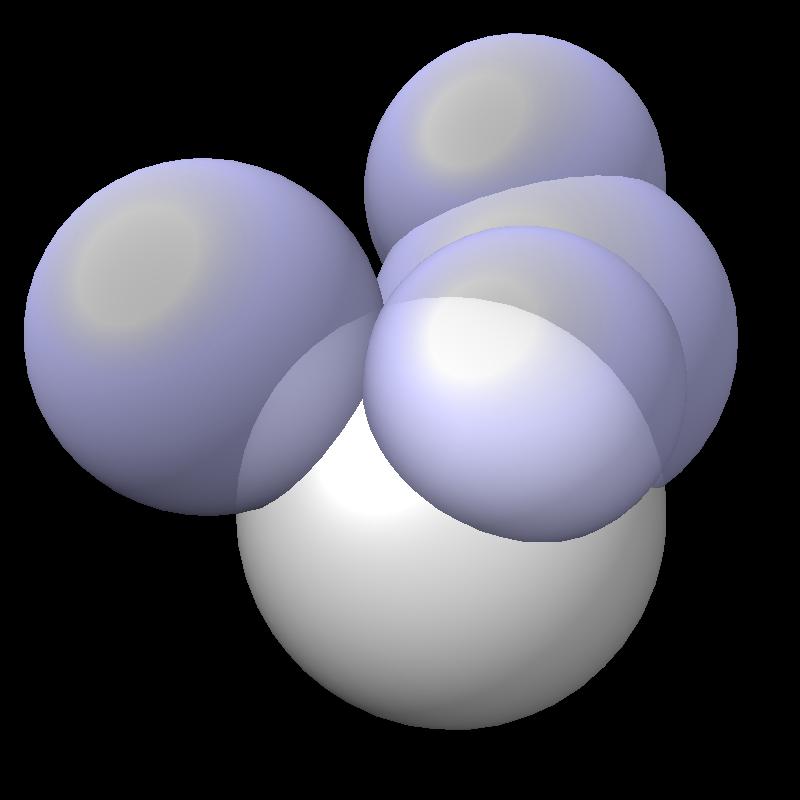
The solvent accessible surface area is the area of the surface swept out by the center of a probe sphere rolling over a molecule (atoms are spheres of varying radii). The solvent accessible surface is just the boundary of the union of atom balls that have their radius increased by the probe radius (typically 1.4 Angstroms). So the accessible area is the surface area of a union of balls.
|
|
|
|
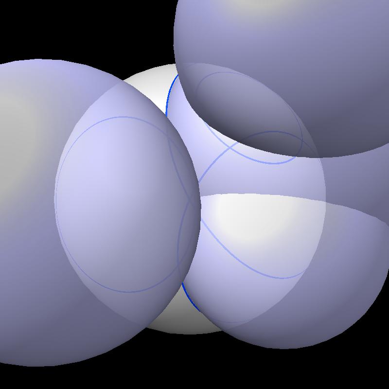
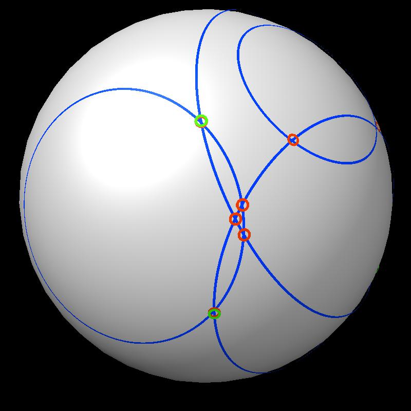
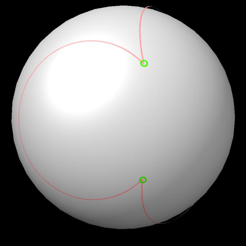
| Find area on gray sphere not inside blue spheres. | Pair of spheres interesects in a circle | Circles intersect each other. |
| 
|
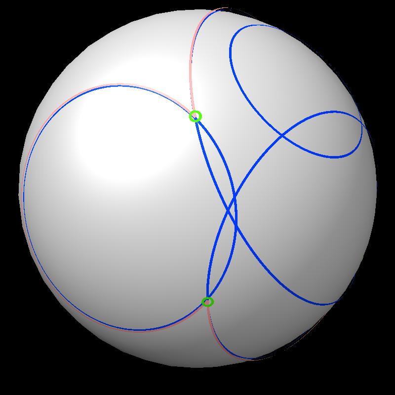
| Boundary intersections of circles (green) | Boundary of union of filled circles (pink) |
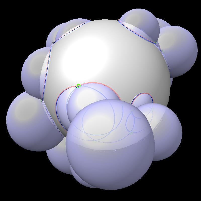
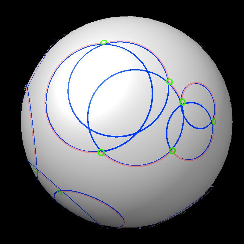
An example with more spheres.
| 
|
| 24 blue spheres | Boundaries have more circular arcs. |
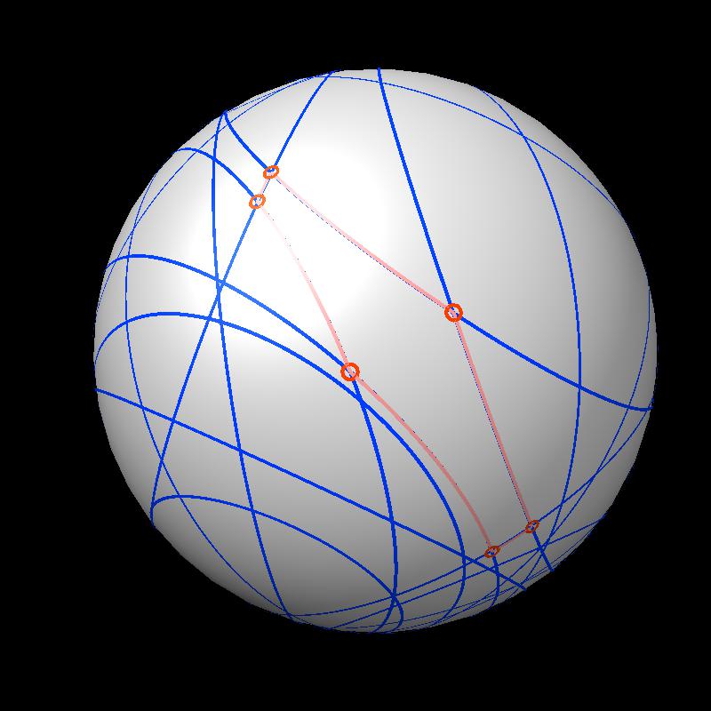
To find the area enclosed by a path on the sphere compute how much the tangent vector to the boundary rotates when traversing the path. Surprisingly the enclosed area if the gray sphere has radius 1 is 2*pi minus the tangent vector rotation angle.
For a circular arc where the circle has angular radius r (in radians), and arc angle a (in radians), the rotation of the tangent vector along the arc is a*cos(r).
If a union of filled circles has more than one boundary loop sum the enclosed areas for each loop and subtract 4*pi*(N-1) for N bounding loops.
To verify that the area calculation based on the piecewise circular boundary curves described above are correct I also calculate a numerical approximation of the area. This works by covering the surface of a sphere with a fine grid of points and counting how many of those points lie inside intersecting spheres. For the set of points I start with the 12 vertices of an icosahedron and then subdivide the 20 triangular faces of the icosahedron into 80 triangular faces by placing a new vertex at the mid-point of each of the 30 edges. Each triangle is subdivided into 4 triangles. Then I repreat this process on the resulting mesh of triangles. The code can subdivide as many times as desired producing 12, 42, 162, 322, 642, 1282 points (= 10*(4^N)+2). I used 642 points for testing. The points are scaled to be distance one from the origin.
The icosahedral subdivision points are not uniformly distributed on a sphere. To correct for that a weighted sum of the points inside other spheres is used. The weight for each point is 1/3 the area of the mesh triangles that share that vertex. These are the triangles formed by the points projected on to the sphere. So the weight is just an area associated with each point.
Using 642 points gave average area error (difference from the analytic area calculation) of about 0.001 times the area of the sphere when tested on Protein DataBank models with 1.4 Angstrom probe radius. The atom with the worst area error typically was off by 0.01 times the area of the sphere.
I ran the analytic and numerical approximation area calculation on all of the molecules in Protein Data Bank (95,280 entries). All calculations succeeded and the analytic and numerical approximations agreed with the atom having the biggest difference in area between anayltic and approximate calculations differing by 0.5 to 2% of full atom sphere area. The total analytic accessible area for all spheres agreed with the numerical estimate to within about 0.1% on average using 642 sample points for the numerical estimate. The exposed area for each atom using a probe radius of 1.4 Angstroms was computed. The radii for each atom were based on the element type (H 1.00, C 1.70, N 1.625, O 1.50, P 1.871, S 1.782, all others 1.5). Water atoms (defined as those in residue named HOH) were excluded. For atoms with alternate locations (ALTLOC) only the first location was used. For multi-model files (NMR ensembles) only the first model was used.
Here is example output, taken from the full output.
Area numerical estimate using 642 sample points per sphere
   PDB  atoms      area     earea atime etime  max err mean err
  100d    422    4130.8    4118.7  0.01  0.02  0.00868  0.00135
  200d    258    2688.5    2688.9  0.00  0.01  0.00720  0.00180
  200l   1299    8593.1    8583.7  0.03  0.07  0.00977  0.00100
  300d    879    7080.6    7073.4  0.02  0.05  0.00784  0.00127
  400d    244    2410.1    2408.2  0.01  0.01  0.00635  0.00129
  101d    520    4460.8    4471.5  0.01  0.03  0.00799  0.00127
  101m   1275    7985.2    7988.3  0.03  0.07  0.01078  0.00099
  201d    911    4798.4    4795.6  0.03  0.05  0.00880  0.00120
  201l   2643   16500.3   16515.4  0.06  0.14  0.01069  0.00095
  301d    878    7282.3    7284.3  0.02  0.05  0.00861  0.00118
...
The 95000 files were processed loading one molecule at a time, calculating areas, than closing that molecule, in the Chimera 2 prototype Hydra. The process apparently had some memory leak and grew to 13 Gbytes of memory use by the end of the 8 hour job.
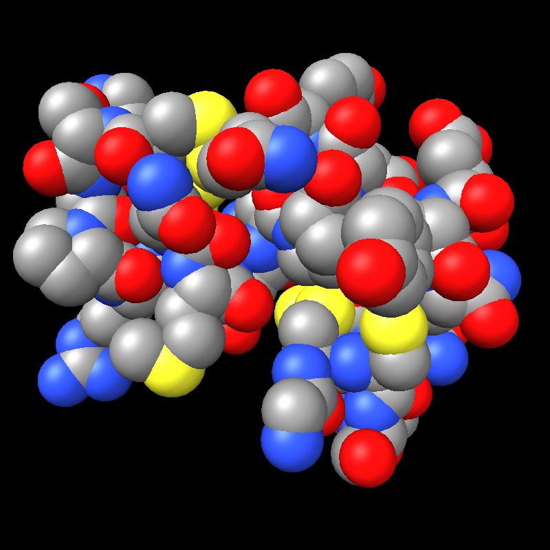
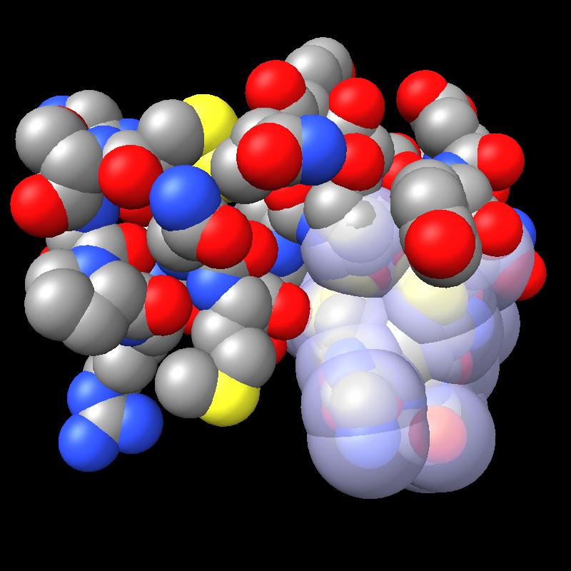
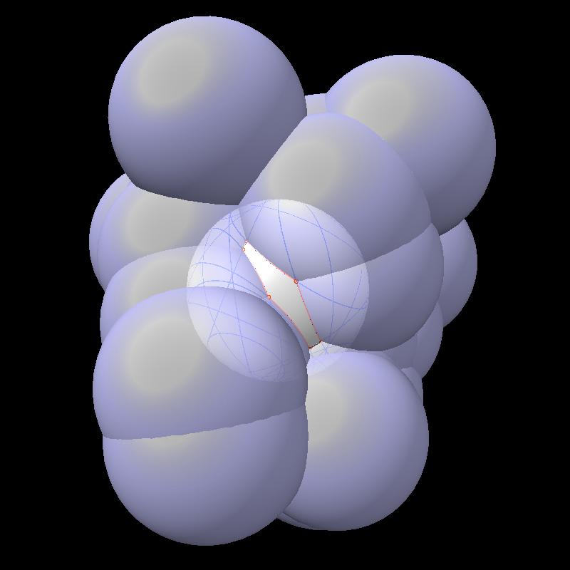
Here are pictures of the accessible area for a single atom of a small protein PDB 1a0m using probe radius 1.4 Angstroms. 39 spheres intersect the atom sphere (extended by one probe radius). 20 of the intersection circles lie completely within another intersection circle. The 19 cirlces that are not inside any other one circle intersect each other in 234 points of which just 6 are on the boundary of the buried region. Much of the area calculation time is to eliminate the intersection points that are buried (not on the boundary).
| 
| 
|
| PDB 1a0m | Atoms plus probe radius intersecting one atom. | 39 spheres intersect chosen sphere. |
| 
|
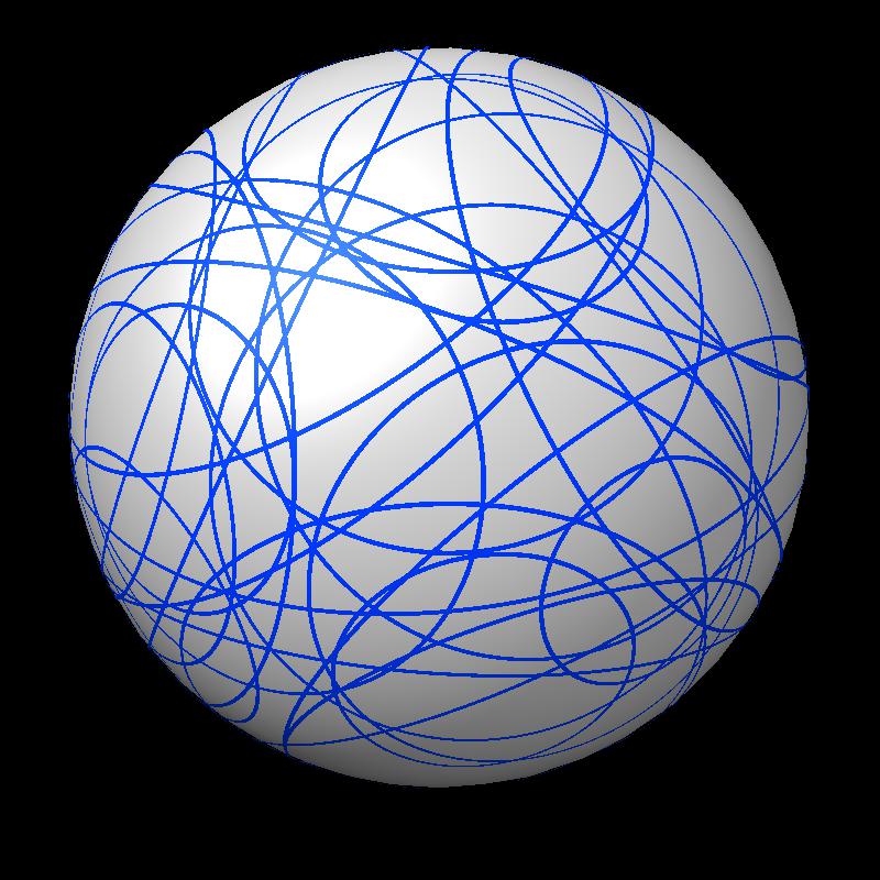
| Outline of exposed region on sphere (pink). | Circles from sphere intersections on opposite side from exposed patch. |
The full PDB calculation took 8.4 hours total wall-clock time, and about 13 hours of CPU time running on 4 cores, and 7.7 hours not including file load times, with 2.4 hours for the analytic computation and 5.3 hours for the numerical approximation. Areas for 510 million atoms were computed averaging about 60,000 atoms per second for the analytic calculation. Large molecules ran faster at about 200,000 atoms per second. This is probably because the parallelized code assigned 100 box regions each containing about 70 atoms to each thread, or about 7000 atoms per thread. So utilizing the 8 hyperthreads (4 cores) requires at least 56,000 atoms.
The spheres close to a given sphere were found more efficiently than an all-by-all distance comparison. Early versions of the code that simply compared distance between sphere centers for all pairs took most of the computation time finding the intersecting spheres for molecules bigger than about 3000 atoms, and for 10,000 atoms that part of the code took about 3 times longer to find contacting spheres then the part that computed the area, and for 100,000 spheres 90% of the computation was finding neighbor spheres. To optimize this I partitioned the spheres into rectangular boxes, by taking the box bounding all spheres and splitting it along the long axis. I successively split the resulting boxes until a box contained at most 100 spheres. I kept a list of the spheres in the box, and those intersecting the box (which includes more spheres near the box boundary). Then I did all-by-all comparisons on these small sets of spheres to find those intersecting each other.
An early, all Python (with numpy) analytic calculation took about 15 seconds for about ~240 atoms of PDB 1a0m, or about 20 atoms per second. The initial C++ implementation processed about 10,000 atoms per second for small (< 1000 atom) molecules and with the optimized nearby sphere code achieved that speed for large molecules also. Some other optimization, maybe culling circles within other circles increased this several fold. Then I parallelized using OpenMP, and achieved the 200,000 atoms on a 4-core i7 iMac typically using 8 threads (twice the number of cores due to Intel hyperthreading).
The analytic calculation is suprisingly slow. I believe the reason for this is that each atom has about n = 50 other atoms that contact it when the probe radius is added to all atom radii. The code computes circles that are the intersections of those 50 spheres with the one sphere. Then it eliminates the many circles contained entirely within other circles taking O(n*n) time. This typically reduces to about m = 20 circles, and all-by-all intersections are done, generating hundreds of intersection points, each of which is tested for inclusion in the 20 circles. That is potentially O(m*m*m) cost, although in practice less since most all intersections are interior points that are found to be within another circle after testing only for inclusion in a few circles. At any rate, profiling and optimization could probably speed the calculation up by a factor of several. Possibly ordering circles, largest radius first might reduce execution time substantially.
A common use of accessible area calculations is to determine buried area. For two sets of spheres the area of each set is computed and then the combined area, then 0.5*(A1 + A2 - A12) is the buried area. This computation can be made much faster by eliminating spheres in each set that are far from all spheres in the other set (greater than twice max radius plus twice probe radius). This is typically a much smaller set of spheres and which spheres to compute can be computed quickly O(NlogN) time with simple methods. This technique could for instance making computing all buried areas between chains of molecular assemblies having many chains take only a fraction of a second.
The analytic area calculation can fail. In this case it will report -1 for the exposed area of a sphere for which the calculation failed. This only happens when the boundary of the buried region cannot be computed. This can happen because which circle intersection points lie on the boundary are incorrectly determined due to round-off errors. In this situation a circle intersection point that is on the boundary may due to roundoff appear inside another sphere, or an interior intersection point may be judged to be on the boundary due to round-off errors. This leads to boundary paths not closing to form loops. An error in determining the boundary is likely to occur if 4 or more spheres intersect at a single point in exact arithmetic. Three spheres intersect in a point, and having a fourth sphere surface coincidentally intersect exactly through such a point is extremely unlikely. The code uses 64-bit floating point math giving about 15 decimal digits of precision. So a random 4 sphere intersection at a single point to within that precision probably occurs only about once in 10^15 placements. Each atom has an exposed area boundary of about 10 circle arcs, so there are about 10 possiblities per atom for coincident intersections. We tested 5*10^8 atoms so only about 5*10^9 chances for coincident intersections, so it is not surpising that we saw no failures in testing the entire PDB. This estimate ignores some of the subtlety of the chance of random coincident intersections, and is just intended as a guess as to the frequency of random failures. Errors would start to appear for intersections points that need not be coincident to 64-bit precision. Close intersections differing only in the last digit or two of precision may lead to such errors. But these rough considerations suggest that thousands of times more atoms than are in the PDB database would be needed to hit a random boundary determination error.
In fact, an earlier calculation included all alternate location (ALTLOC) atom positions in computing the surface area and there was one PDB structure with boundary determination failures for 12 atoms, PDB 3b2c. Inspection showed that the structure has 7 alternate atom locations for every atoms and many of the alternate positions are 0.001 Angstroms away from other alternate positions, 0.001 being the precision of numbers specified in the PDB files. This put many atoms next to each other on an exact grid with 0.001 spacing which led to coincident intersections. When areas were computed using just one position for each atom the area calculation worked without failures.
Since the boundary determination failure is detected, the area for that sphere could then be computed with the numerical approximation, and a warning issued. Or the boundary circles could be perturbed by a small amount comparable to the floating point precision and recomputation done. It is possible that one or more boundary determination errors occur for circles on a sphere and the result is a consistent (closed loop) boundary but not the correct boundary. These could be hard to catch and could possibly lead to a large area error, but are expected to be much rarer than inconsistent boundary cases.
Here is a C++ implementation of the area calculation: sas_area.cpp. On Mac OS 10.8 I compile and run it with
$ c++ sas_area.cpp -o sasa
$ ./sasa
Computed SAS area for 10 spheres, 10 successful, total area = 8.76967
 estimated with 10000 points per sphere, total area = 8.78171
Early versions of the surface area calculation code crashed into many unpleasant PDB entries.