Chimera Workshop
November 17-18, 2005
This tutorial shows how to work with volume data in Chimera. Volume data means a 3-dimensional grid of data values.
We'll look at three kinds of volume data:
|
|
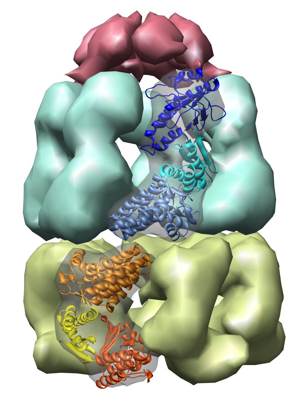
| Figure 1: E coli chaperonin shown using the Chimera MultiScale tool. The top red cap is GroES, the blue and yellow rings are GroEL. Protein Data Bank model 1AON. |
The examples will all involve a 21 protein molecular complex called chaperonin. Chaperonin is a barrel inside which proteins are folded. In bacteria it consists of 3 rings each containing 7 proteins. Two rings of 14 identical proteins form a barrel called GroEL. The cap, called GroES, is formed from 7 copies of a different protein.
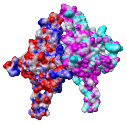
We will color a molecular surface to show electrostatic potential.
Open in Chimera the Mycobacterium tuberculosis GroES structure. The protein data bank model 1p3h contains two copies of GroES but the file you've opened contains just one copy.
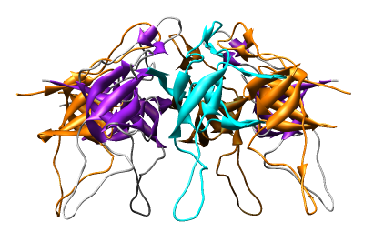
Change from an all-atom view to a round ribbon display. You can use menu entries:
The 7 proteins can be given different colors.
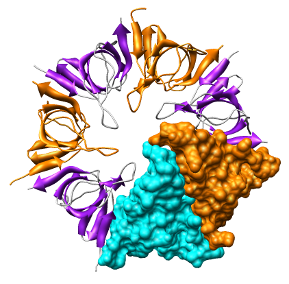
Create a molecular surface for chain A. The Actions menu allows you to make a single surface covering all 7 chains, but to surface just one requires using Chimera commands:
To color the molecular surface according to electrostatic potential.
The file 1p3h_chain_A.nc is electrostatic potential volume data calculated by the Adaptive Poisson Boltzmann Solver (APBS) for chain A outside of Chimera. Chimera is not able to calculate the potential itself. Running APBS is not part of this tutorial.
The colors represent potential values, blue at potential 10 kT/e, red at -10 kT/e, and white at 0 kT/e, with linear interpolation of colors at intermediate potential values.
Repeat the surface display and electrostatics coloring steps for chain B to see the electrostatic potential on the neighboring monomer. In the Surface Color dialog you will need to choose to color MSMS b surface and use the potential file 1p3h_chain_B.nc that was calculated for chain B.
Pressing the red and blue color buttons on the Surface Color dialog you can change the surface colors. Then press the Color button at the bottom of the Surface Color dialog to apply these new colors. That will help visually distinguish the surfaces for chains A and B.
Are the potential values for chains A and B at their interface complementary, that is, positive on one side and negative on the other?
The GroES model above was determined by x-ray crystallography. We'll now look at the agreement between the atomic model and the x-ray density map.
First clean up from the previous electrostatics example.
Open the 2.8 angstrom resolution crystallographic density map 1p3h.omap which came from the Uppsala Electron Density Server web site.
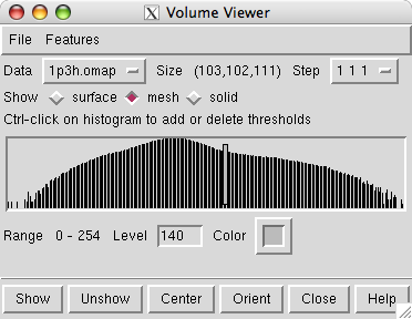
Opening the density map causes the Volume Viewer dialog to be displayed. It shows that the map grid is of size 103 by 102 by 111 and a histogram of the density values is shown. The vertical bar on the histogram indicates the currently displayed surface contour level. The bar can be moved with the mouse to change the contour level. The initial step setting is 2 2 2 indicating that every other plane of the data is being displayed.
Adjust some density map display settings.

To compare the density map and model it is necessary to look at a small piece. We'll look at the density near chain A.
Show chain A atoms and hide all other chains.
See what types of residues are sticking out of the density map.
Long side chains like lysines, arginines and glutamic acid on the surface probably assume variable positions in the crystal. Their exact positions in the model should not be trusted.
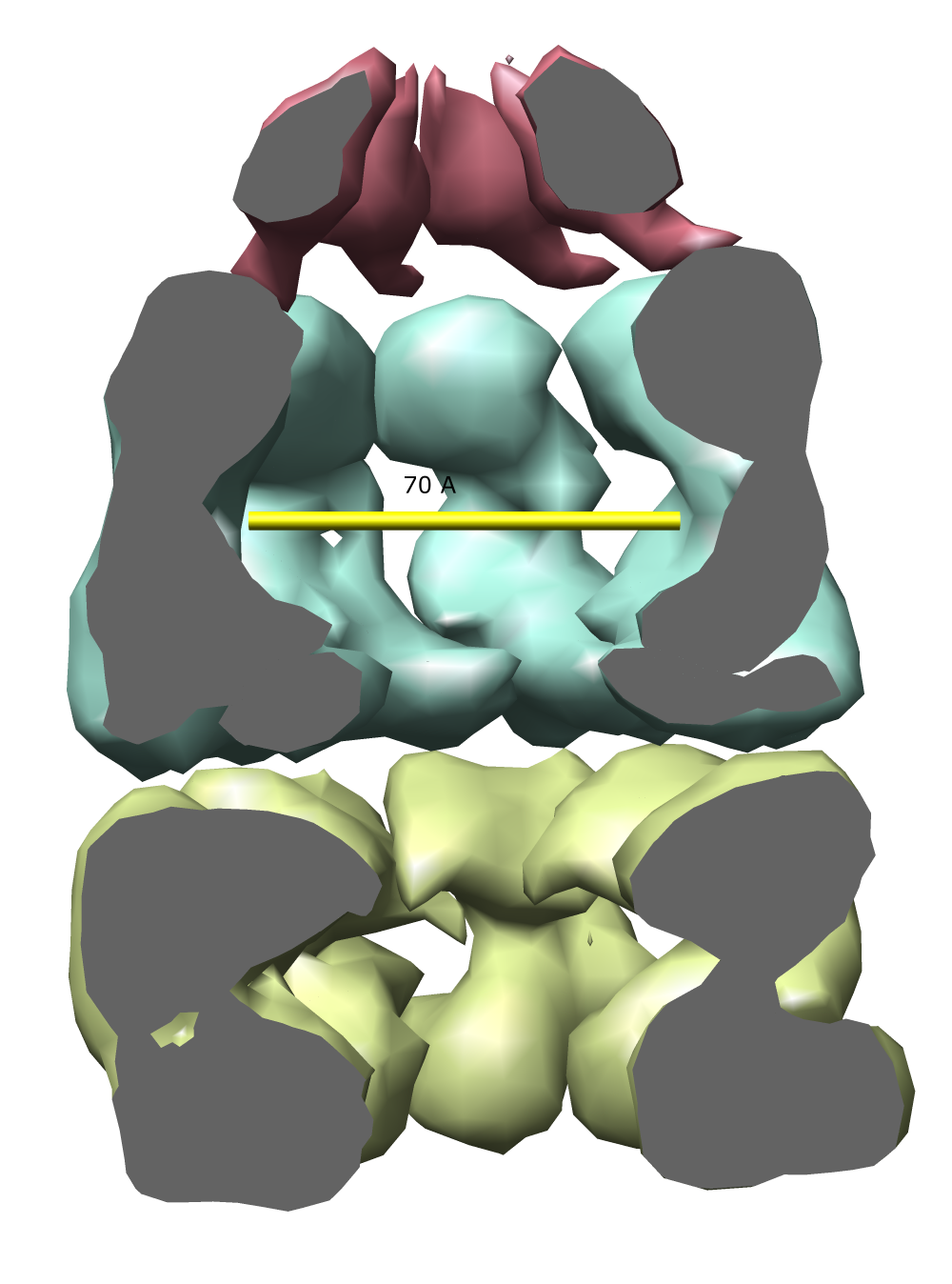
Now we will try fitting a protein into a density map of E coli chaperonin determined by electron microscopy.
Clean up from the previous x-ray density map example.
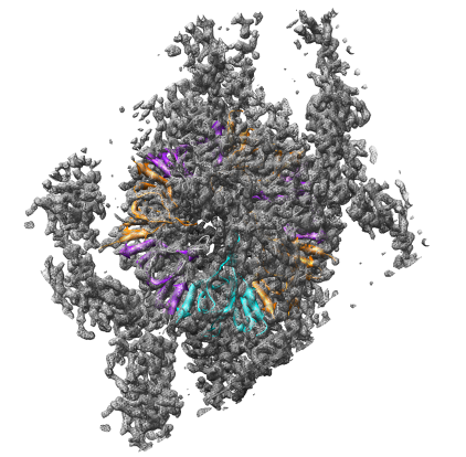
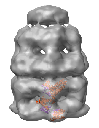
Open the 23.5 angstrom chaperonin density map which was determined by single particle reconstruction using 2-D electron micrographs of 1448 particles, and the 2.8 angstrom GroEL protein crystal structure.
Adjust the map contour level and step size and display style in the volume dialog.
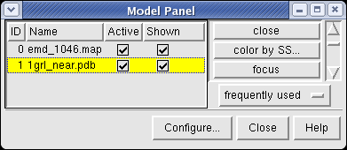
Show the molecule as a ribbon colored according to secondary structure (alpha helices orange, sheets purple).
|
|
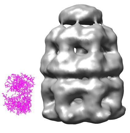
Lock the position of the density map and move the molecule into the map using the mouse.
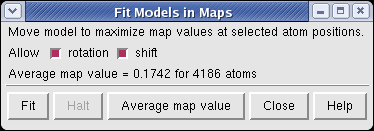
The molecule can be automatically moved to the nearby position that maximizes the density values at atom positions.
Fitting the molecule upside down gives an average density value at atom positions of 0.167, while the correct orientation gives 0.174.