Drug Network Fusion

Integrative Cancer Pharmacogenomics to Infer Large-Scale Drug Taxonomy. El-Hachem N, Gendoo DMA, Ghoraie LS, Safikhani Z, Smirnov P, Chung C, Deng K, Fang A, Birkwood E, Ho C, Isserlin R, Bader GD, Goldenberg A, Haibe-Kains B. Cancer Res. 2017 Jun 1;77(11):3057-3069. PMID: 28314784
Web application: http://dnf.pmgenomics.ca
Code: https://github.com/bhklab/DrugNetworkFusion

Summary

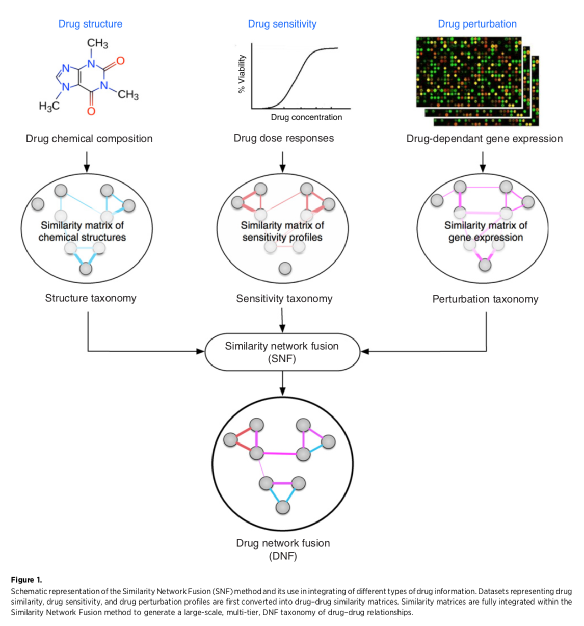
1. construct three separate networks of “drugs” (compounds) with edges based on similarities in:
   • drug structure - Tanimoto similarity calculated from SMILES; extended connectivity fingerprint also mentioned but unclear if/how it was used
   • sensitivities of cancer cell lines to drug - Pearson correlation of sensitivity profiles, two datasets tried separately:
     • National Cancer Institute NCI60: 60 cell lines x >40,000 compounds, Z-score metric
     • Cancer Therapy Response Portal CTRPv2: 860 cell lines x 481 compounds, AUC metric
   • expression perturbation of cancer cell lines - Pearson correlation of drug-effect-on-gene coefficients from linear regression (including treatment duration, cell-line identity, and batch in addition to drug concentration)
     • NIH Library of Integrated Network-based Cellular Signatures (LINCS) L1000 (also used in Hetionet/SPOKE): ~1000 genes x >20,000 compounds
2. “fuse” those three into a single network
3. see how well the single network classifies drugs

Fig 1: Creating the drug network fusion (DNF)

Network Fusion

Similarity network fusion for aggregating data types on a genomic scale. Wang B, Mezlini AM, Demir F, Fiume M, Tu Z, Brudno M, Haibe-Kains B, Goldenberg A. Nat Methods. 2014 Mar;11(3):333-7. PMID: 24464287
Code: http://compbio.cs.toronto.edu/SNF/

1. generate node similarity matrix for each data type
2. iterate (method is nonlinear, based on message-passing theory) to make each network more similar to the others
3. convergence is single fused network

Evaluation

Calculate ROC (edge weight in fused network as continuous variable) for identifying compounds that share a target or therapeutic category:

• target - from DrugBank for NCI60, from CTRPv2 website for that dataset
• therapeutic class - Anatomic Therapeutic Classification (ATC) codes from ChEMBL for drugs common to NCI60 and CTRPv2; ATC level 4 describes the chemical, therapeutic, and pharmacologic subgroup of a drug

Fig 2: The fused network is better than the single-data-type networks at grouping drugs by target or class

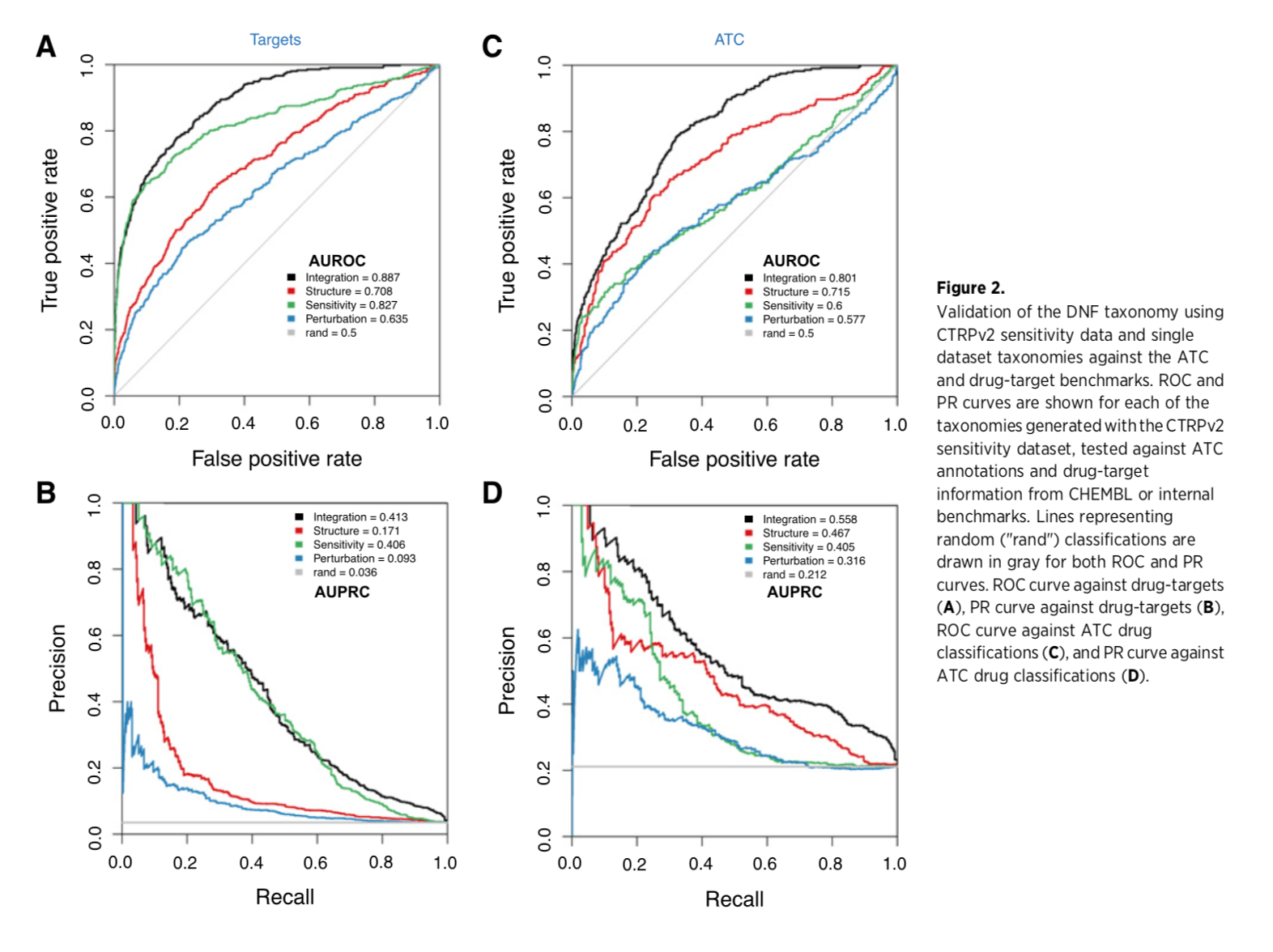
(Supplementary data also includes comparisons with four published methods of drug classification, with the DNF outperforming each one.)

Clustering the DNF

Clustering was done by affinity propagation. Each community is represented by an “exemplar” compound. The NCI60 fusion includes 238 drugs, 51 communities. The CTRP fusion includes 239 drugs, 53 communities.

Web app screenshot: CTRP exemplar network

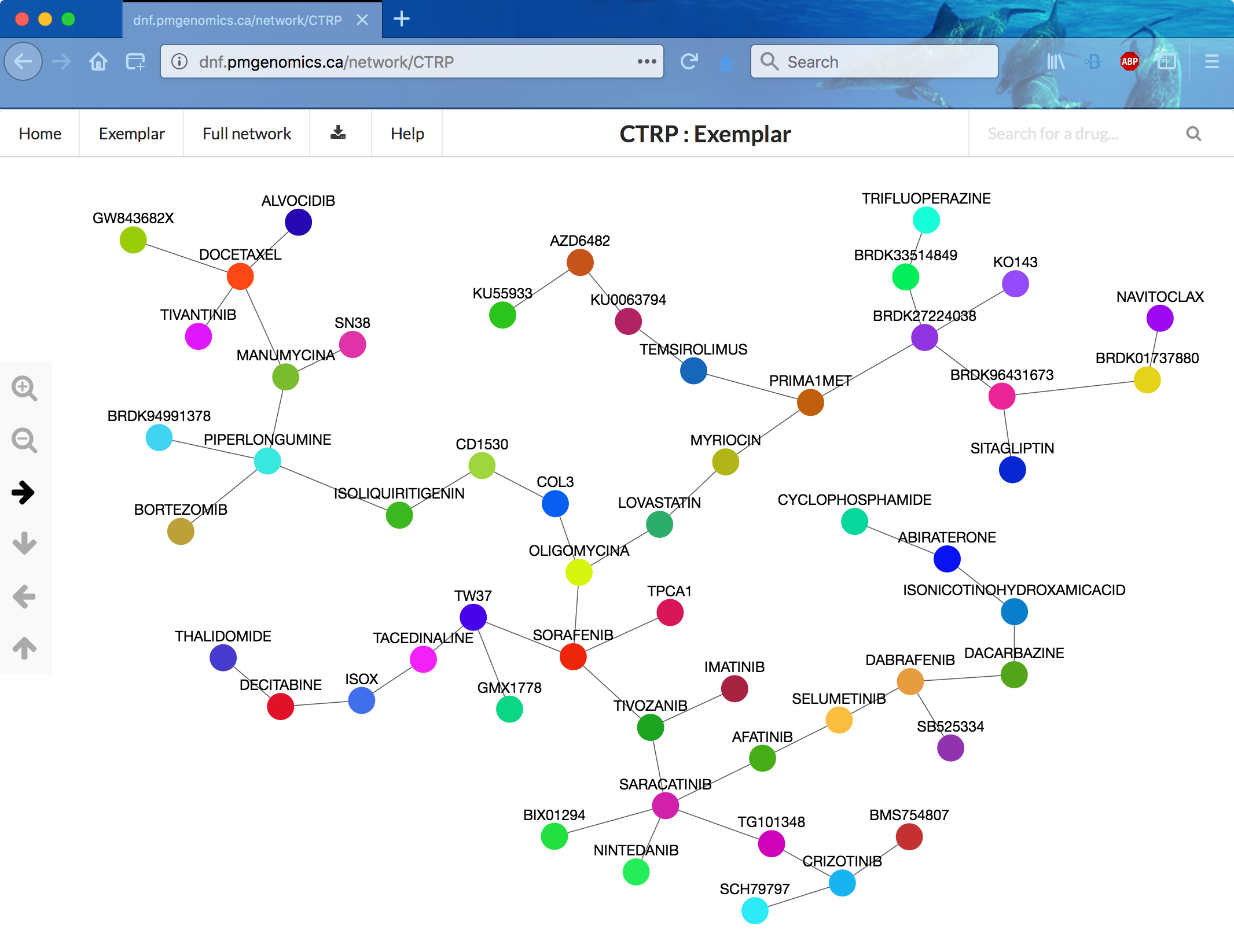
DNF Web app

http://dnf.pmgenomics.ca

• frontend implemented using JavaScript and AngularJS
• backend implemented using Node.js
• network information stored as JSON
• graph rendered with the Cytoscape.js library, thresholded to show the top 1000 edges of the full networks
• chemical diagrams (just in the paper?) drawn with Cytoscape chemViz

Choices to view are the two fusion networks (CTRP or NCI60 data), each as the full network or the exemplar minimal spanning tree. The landing page was very slow to appear (~3 min?), but after that, I could view and navigate the networks without lags (although the arrows seem backwards), expand exemplars to their communities, and show detailed information for nodes and edges. Clicking an edge shows the relative contributions of the three data types as a donut chart.

Limitations given in the paper

• limited overlap between sensitivity and perturbation data (i.e., not that many compounds in common... apparently <240!)
• unclear how best to normalize L1000 (perturbation) data
• unclear how best to measure similarity in sensitivity profiles
• heterogeneity in sensitivity data (NCI60 and CTRP report different things)
• comparisons with other resources not very thorough because of limited overlap with those resources

...however, they contend that the amount of data is increasing and that more compounds could be clustered with DNF, given:

• canonical SMILES string
• list of genes perturbed by the compound in at least three cell lines (genome-wide transcriptional studies preferred to maximize overlap with L1000)
• sensitivity profiles including measurements of cell growth at nine compound concentrations for at least 50 cell lines from multiple tissues

Discussion/Critique

• The salient difference from heterogeneous networks is that fusion networks only have one kind of node (only the edges are fused): patients in the 2014 SNF paper, drugs in this paper.
• Is there a practical limit on how many types of similarity data can be combined? These studies each used three types.
• Maybe a fusion network could be incorporated into a heterogeneous network, but would that be useful?
• Are some data types too orthogonal to fuse? The authors say their data types were complementary. The SNF paper suggests using normalized mutual information (NMI) to clarify which datasets may be combined fruitfully.
• Does this DNF provide new information? A few interesting examples were given. Maybe even when primary targets are known or suspected, the network can reveal commonalities in side or downstream targets, or the existence of larger systems involving the known target.
• The application to classify cancer patients (2014 paper) may be more promising, given the data limitations for drugs.

Benchmarking Molecular Networks for Disease-Gene Identification

Systematic Evaluation of Molecular Networks for Discovery of Disease Genes Huang JK, Carlin DE, Yu MK, Zhang W, Kreisberg JF, Tamayo P, Ideker T. Cell Syst. 2018 Apr 25;6(4):484-495.e5. PMID: 29605183

Network Types and Evaluation Task

• evaluated 21 publicly available human gene interaction networks
• “interaction” being a catch-all term encompassing direct binding, genetic interactions, expression correlation, etc.
• varying levels of evidence, from experiments reported in the literature to computational inference
• candidate disease genes identified by network proximity to known disease genes

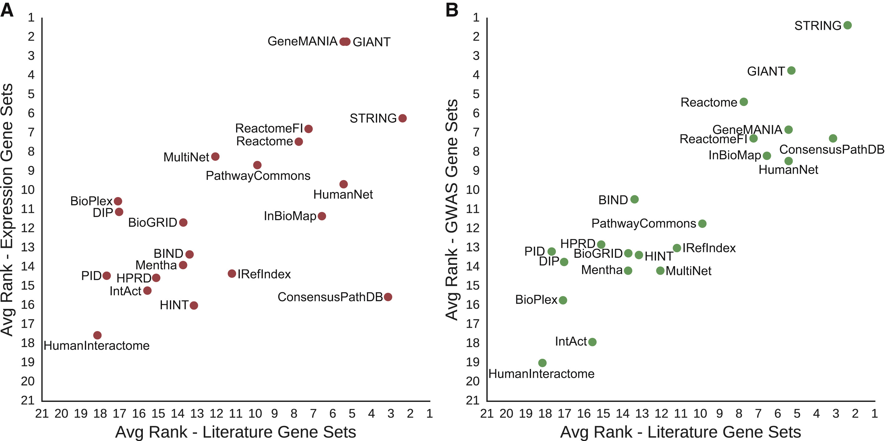
Fig 1: Summary of Networks Evaluated

“Specific interaction content varied widely, even among repositories that appeared superficially similar.”

Gray X means excluded from this evaluation because of some data issue.

Evaluation

Using 446 disease-associated gene sets (literature gene sets) from DisGeNET:

1. in a given network, randomly split the gene set of interest into two subsets
2. try to recover one subset by network propagation from the other (random walk with restart)
3. calculate area under precision-recall curve (AUPRC), average over multiple trials
4. performance score = Z-score vs. null AUPRC from shuffled-edge networks
5. controls did not change conclusions:
   • remove all non-disease genes from network first
   • use an effect size metric, performance gain (in case of Z-scores being large due to low null-model variance)

Fig 2: Evaluation Schematic

• proportion to sample based on number of genes from that set in the network
• amount of network propagation based on number of edges in the network

Fig 3: Performance

• all 21 outperformed their null models on at least 49% of the gene sets
• 26% of gene sets recovered at a Bonferroni-corrected p-value <0.05 by all 21
• larger networks better, STRING best overall
• other network characteristics not significantly correlated with performance

Controls for Literature Evidence

...since DisGeNET is based on text mining, wanted to see if networks with that kind of edge had an unfair advantage...

• removing text-mining edges significantly decreased the performance of HumanNet (~1% of edges) but not that of STRING (~12% of edges)
• using non-literature-based disease gene sets for evaluation did not change the results very much (Fig. 4)
  • 9 cancer gene sets from mRNA profiling data – GIANT and GeneMANIA best, but STRING third
  • 9 disease gene sets and 2 for complex traits (height, body mass) from GWAS

If Larger is Better, Try Combining Networks

• simple agglomeration did not improve performance (Fig 5A)
• removing edges that only came from one network (giving the Parsimonious Composite Network, PCNet) improved performance beyond STRING even though PCNet was much smaller (Fig 5B)
• requiring support from >2 networks degraded performance

• A: additive combined networks
• B: parsimonious filtering of largest combined network
• performance gain (---- STRING alone)
• # edges (---- STRING alone)

Pathogenic Gene Prediction by Multipath Random Walking on Heterogeneous Network

A network embedding model for pathogenic genes prediction by multi-path random walking on heterogeneous network. Xu B, Liu Y, Yu S, Wang L, Dong J, Lin H, Yang Z, Wang J, Xia F. BMC Med Genomics. 2019 Dec 23;12(Suppl 10):188. doi: 10.1186/s12920-019-0627-z. PMID: 31865919

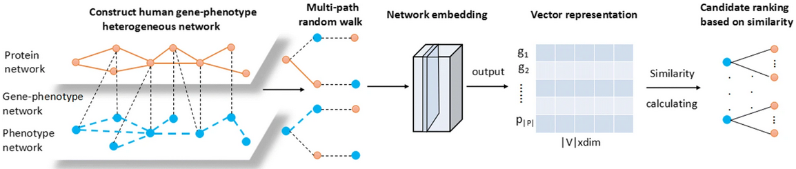
Multipath2vec method to predict pathogenic genes:

1. create “GP-network” from three kinds of relationships (to them, Gene = protein, Phenotype = disease):
   • G-G interactions: from the Human Protein Reference Database, PPIs involving 8756 proteins
   • P-P correlations: cosine similarities > 0.6 from the 5080x5080 matrix available from MimMiner
   • G-P pairs from OMIM, initially 925 involving 667 pathogenic genes and 775 disease phenotypes, but then filtering out those with genes or proteins not present in the other datasets
2. perform multipath random walk
3. learn an embedding using heterogeneous skip-gram
4. normalize the resulting vectors and rank by similarity, i.e., rank gene vectors by cosine similarity to the phenotype vector for a disease of interest

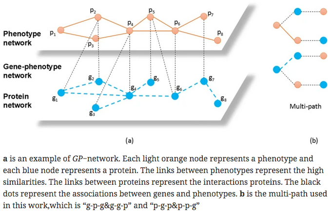
• previous work derived vectors from metapaths along g-p edges only
• this work derives vectors from multipaths that also include g-g and p-p edges (but not g-g-g or p-p-p)
• I didn't understand the embedding from metapaths to vectors. Scooter says it is based on the skip-gram machine learning approach to predict the context words for a given target word, developed primarily for natural language processing.

Other methods compared with Multipath2vec:

• Metapath2vec – g-p-g walks only (no g-g, p-p)
• Deepwalk – uniform random walks treating all node types equally
• CATAPULT – bagging SVM generates a linear classifier from the numbers of paths of different lengths for a gene-protein pair
• PRINCE – gene-disease correlation based on a priori knowledge of the gene and correlation between its neighboring genes and the disease

Comparison was by leave-one-out cross-validation, with Multipath2vec settings:

• 500 walks per vertex
• walk length 100
• neighborhood size 7
• 5 negative samples
• vector length 128

They only reported precision TP/(TP + FP). However, they claimed “the number of TP is equal to the number of TN and the number of FP is equal to the number of FN. Our method perform well in the accuracy of prediction, so it is also robust to false negative.”

The distinction between their three types of comparison, “single-genes, many-genes and whole-genes gene-phenotype data,” was not explained. The whole-genes results were intermediate between the two shown here:

single-genes gene-phenotype data	many-genes gene-phenotype data

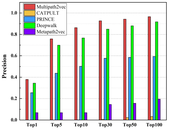
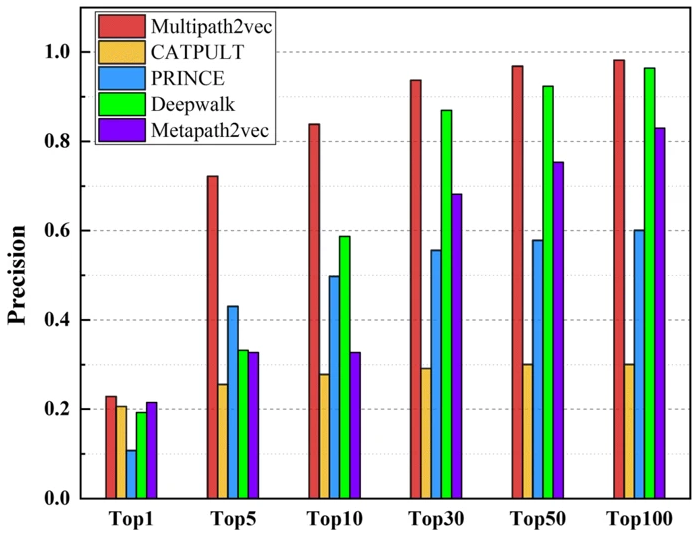
In most comparisons Multipath2vec was the best but only slightly better than Deepwalk. Code was not provided.

Pathway and Network Embedding Methods for Prioritizing Psychiatric Drugs

Pathway and network embedding methods for prioritizing psychiatric drugs. Pershad Y, Guo M, Altman RB. Pac Symp Biocomput. 2020;25:671-682. PMID: 31797637

Motivation

“ ...nearly 75% of psychiatric prescriptions do not successfully treat the patient's condition.”

“Understanding the molecular basis of psychiatric diseases is necessary for rational drug choice... Gene expression levels provide quantitative measures to characterize these disrupted molecular pathways... Previous work has analyzed gene expression data to find novel disease-gene associations and has even predicted non-psychiatric diseases via PPI networks and pathway-based approaches. The advantage of these network approaches is that they maintain a higher degree of biological interpretability compared to models using gene expression data directly as features.”

Definitions

• disease module – a group of connected genes likely associated with the same disease
• drug module – a group of connected genes likely known to be targets of a drug
• (however, they use signature is as a synonym for module, and their method does not require the genes to form a single connected group)
• embedding – capturing the complex relationships between network nodes in a lower-dimensional space
• node2vec – type of embedding expressed as a feature vector for each node

Data Collection

1. expression data obtained from Gene Expression Omnibus (GEO) for 145 cases of schizophrenia, 82 cases of bipolar disorder, 190 cases of major depressive disorder, and 307 shared controls
2. genes mapped to multiple probes were averaged
3. data were normalized and corrected for batch effects

Predicting Disease from Expression Data

1. PCA, UMAP (uniform manifold approximation and projection), and unsupervised learning methods based on 2D visualization of feature vectors were evaluated for distinguishing the diseases from expression data
   • UMAP did not show clustering by disease (others not mentioned)
2. PROPS (Probabilistic Pathway Score) was used to identify KEGG pathways enriched in each disease sample as compared to a control sample
3. Classifiers were trained to distinguish the diseases from one another using the PROPS pathway scores as features
   • Performance: random forest (auROC avg. 0.78) > support vector > decision tree
4. The most important pathway features of the random forest model were identified and gene importance inferred from frequency of association with high-scoring pathways
5. Genes from the 20 most important KEGG pathways for each disease were added to “augment” a disease signature (described below) if not already in the signature of another disease

Ranking Disease-Relevant Drugs

1. Initial disease signatures (disease-associated gene sets) for bipolar disorder, MDD, and schizophrenia were obtained from Psychiatric disorders and Genes association NETwork (PsyGeNET), an expert-curated database based on DisGeNET and literature mining
2. Genes with significant SNPs for the respective diseases in GWAS Catalog were added to the signatures (444 for bipolar disorder, 892 for MDD, 1261 for schizophrenia)
3. GO molecular-function enrichment analysis was performed for each disease signature vs. all genes with molecular functions in GO and in Reactome pathways
4. Drug targets for 275 psychiatric drugs were obtained from:
   • expertly curated lists – DrugCentral, Drug-Gene Interaction Database
   • literature mining – chemical-gene relationships from the Global Network of Biomedical Relationships (GNBR) derived from PubMed abstracts (also contains diseases; several versions on Zenodo, latest Sep 2019)
   • gene expression signatures – from Connectivity Map (CMap), genes differentially expressed before and after small-molecule treatment (score magnitude > 8)
5. Seven methods of evaluating the similarity between a disease module (from #1-3 above, +/– “augmentation”) and a drug module (from #4) were compared...

Seven Methods to Rank Drugs for a Disease

1. random – simply the proportion of drugs in the total list that treat that disease
2. simple overlap – Jaccard similarity = shared/(total in both sets) × 100%
3. connected components – Jaccard similarity after adding the genes in the shortest path in the STRING v10 PPI network (hereafter “String”) connecting each pair of genes in the disease module
4. mean path length – average path length for a drug after identifying the shortest path in String from each drug-module gene to each disease-module gene (shortest length means strongest similarity)
5. GNBR32D – mean cosine similarity of each pairwise combination of drug-module and disease-module genes after node2vec embedding of GNBR into 32 dimensions
6. String32D – mean cosine similarity of each pairwise combination of drug-module and disease-module genes after node2vec embedding of String into 32 dimensions
7. String64D – mean cosine similarity of each pairwise combination of drug-module and disease-module genes after node2vec embedding of String into 64 dimensions

The top 25 drugs for each disease according to each method were compared to their labeled indications as taken from the Side Effect Resource (SIDER) database.

Drug-disease module overlap is at least slightly greater than random, and node2vec embeddings of PPI networks (methods #6-7) best prioritized disease-relevant drugs (Fig 3A). Embedding methods may better capture the latent neighborhood structure in the network. Disease signatures augmented with pathway-relevant genes outperformed the initial signatures (Fig 3B).

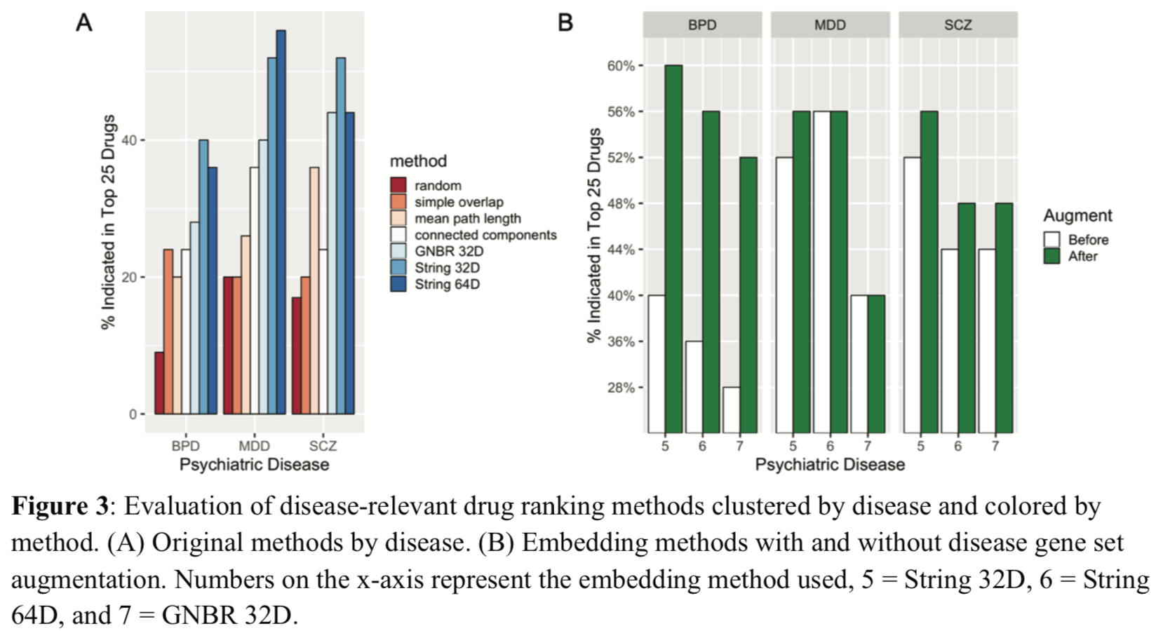
Augmenting increased BPD and SCZ signatures by ~200 genes each, MDD by fewer than 20. Adding 250 random genes gave poor performance.

Some predicted/suggested treatments that are not currently approved have at least semi-plausible explanations:

• niflumic acid for major depression – COX-2 inhibitor used for pain/arthritis in Europe, but other activities include effects on chloride channels and GABA-A and NMDA receptors. Recently approved ketamine also inhibits the NMDA receptor.
  
  
• chlorzoxazone for schizophrenia – used as muscle relaxant/antispasmodic, may activate sodium-activated potassium channels. Low activity of these channels may be implicated in schizophrenia.

I didn't think this figure was as interesting as the authors seemed to think.

They said: The original signatures have similar enriched Reactome pathways to each other, suggesting common mechanisms across the diseases. However, there are some differences in the enriched pathways of the augmented signatures.

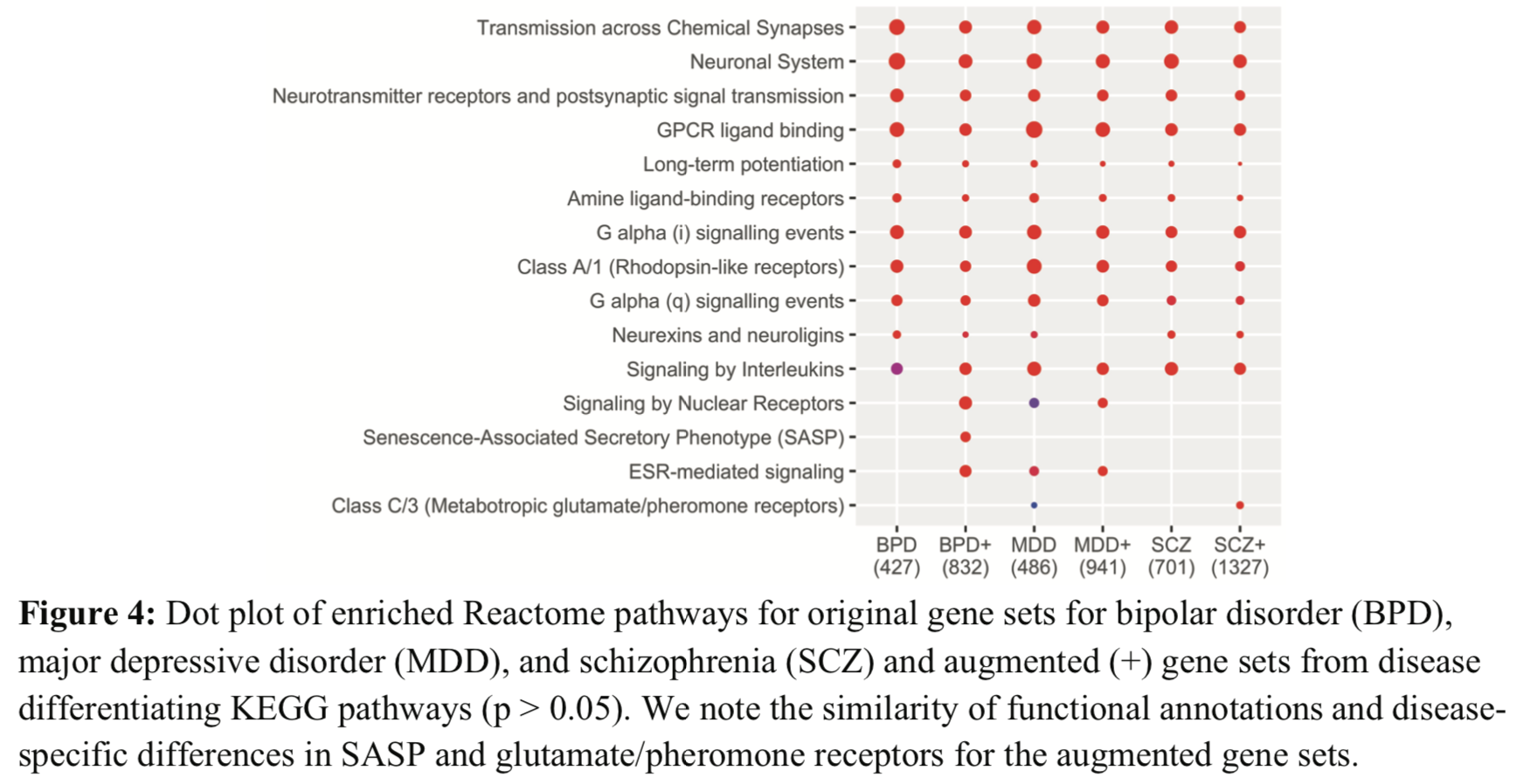
If the numbers in parentheses are the numbers of genes, they disagree with the previous statements of how many genes were added by augmentation. Are they the numbers of pathways? (seem high for that)

Extracting Medical Knowledge from EHRs

Robustly Extracting Medical Knowledge from EHRs: A Case Study of Learning a Health Knowledge Graph. Chen IY, Agrawal M, Horng S, Sontag D. Pac Symp Biocomput. 2020;25:19-30. PMID: 31797583 [supplementary PDF]

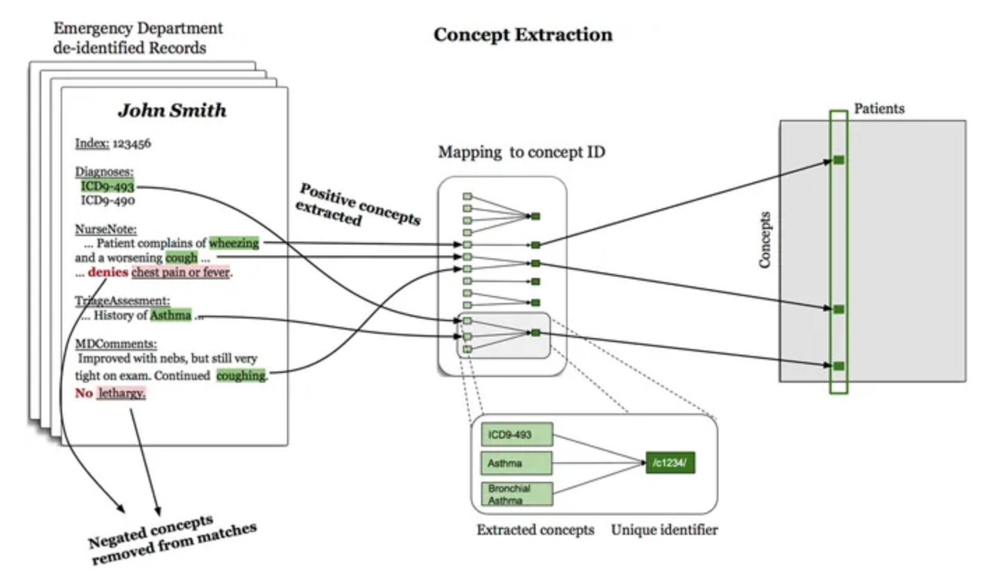
Electronic health records (EHRs) are a rich source of information, but mining them effectively is a complex problem. This paper analyzes a health knowledge graph (diseases + symptoms) previously derived from records of >270,000 emergency department visits.

Aims of Study

• Evaluate our previously constructed symptom-disease network to understand for which patients and which diseases automated extraction from EHRs is most (and least) successful by comparison to a gold standard network.
   
  
• Identify potential confounders and analyze errors to improve building networks for use as diagnostic tools and to better understand diseases.
   
  
• Try alternative statistical models and datasets to see if they yield an improved network as compared to the gold standard.

Gold Standard Dataset

The manually curated Google Health Knowledge Graph (GHKG) is used as the gold standard for evaluation.

The existence of a disease-symptom edge in a proposed health knowledge graph is compared to that in the GHKG to calculate precision and recall. For assessing health knowledge graphs recovered by likelihood estimation, we use the area under the precision-recall curve (AUPRC). For each disease, we include the same number of edges as in the GHKG. Pain was removed from the available symptoms because of inconsistent inclusion in the GHKG.

I note that Yahoo search for GHKG gave as the top hit a critical blog entry. Google search gave a more neutral description.

Data Extraction in the Previous Work

Learning a Health Knowledge Graph from Electronic Medical Records. Rotmensch M, Halpern Y, Tlimat A, Horng S, Sontag D. Sci Rep. 2017 Jul 20;7(1):5994.

“The set of diseases and symptoms considered were chosen from the GHKG... We used string-matching to search for concepts via their common names, aliases or acronyms, where aliases and acronyms were obtained both from the GHKG and UMLS for diseases where the mapping was known... Similarly, if a link to an ICD-9 code was provided, we searched for that code in the record’s structured administrative data. A modified version of NegEx was used to find negation scopes... Mentions that occured within a negation scope were not counted.”

Previously Derived Graph

The previous health knowledge graph was constructed using three different statistical models, with edges drawn between disease and symptom nodes for which the importance metric exceeded a threshold chosen for that model.

• logistic regression, with the metric being the weight of the symptom in a regression fit to predict the disease
• naive Bayes, importance metric related to the probability of disease given the symptom
• noisy OR, importance metric related to the probability of the symptom given the disease (the best of the three models, as shown in Tables 2,5 on later slides)

Datasets

• ED: patient de-identified records from 273,174 visits (by 140,804 patients) to the Emergency Department of Beth Israel Deaconess Medical Center (Boston) between 2008 and 2013; these were used in the previous work to construct the health knowledge graph.
• CR: complete records for the same 140,804 patients as in the ED dataset, aggregated in three different ways:
  • each note taken separately: 7,401,040 instances
  • per patient episode, chained together if separated by ≤ 30 days: 1,481,283
  • per patient, median number of notes 13, median timespan 2.5 years

  Positive mentions of 192 possible diseases and 771 possible symptoms were extracted from both datasets. For each ED visit or CR episode, the mentions are stored as binary variables. For the ED dataset, concepts were extracted from structured data (e.g., ICD-9 diagnosis codes) as well as unstructured, and for the CR dataset, from unstructured notes only.

  We defined sufficient support in the entire dataset for a disease as ≥ 100 positive mentions and for a symptom as ≥ 10 positive mentions. For the ED dataset, this gave 156 diseases and 491 symptoms, and the same diseases and symptoms were extracted from the CR dataset. Age and gender were taken from the ED admission records.

Predicting Individual Diseases

For each disease, we sort symptoms by their importance scores and include the top 25 symptoms in the health knowledge graph (here, from noisy OR) as a binary edge between disease and symptom. The existence of an edge between a given disease and all possible symptoms is compared to that in the gold standard. The harmonic mean of the resulting precision and recall values is the F1 score for that disease.

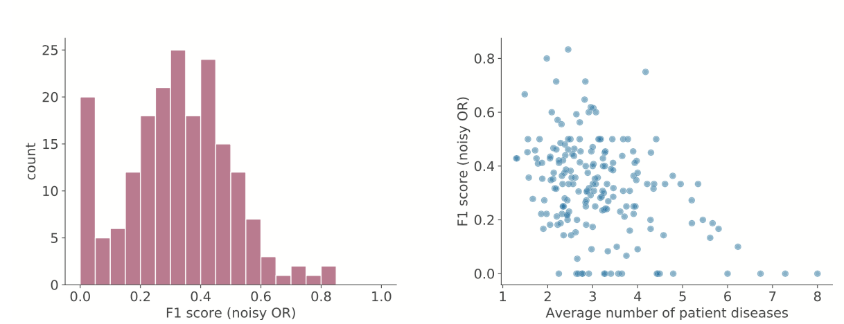
Left: distribution of F1 scores for diseases. Right: F1 scores decrease for diseases that have patients with many co-occurring diseases; the multiple diseases may be reducing the signal that noisy OR can learn.

Including Demographics

Diseases with lower F1 scores are more likely to have more co-occurring diseases and symptoms, more extremely low or high ages, and more extremely low or high % female (Table 1, not shown), suggesting it might be useful to include demographic variables.

However, Table 2 shows that neither using the nonlinear method (causal) nor including age and gender (demo) gives much if any improvement:

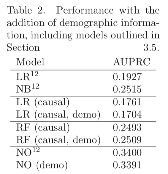
(p. 25, but conflicting statement on p. 21? “demographic data improves performance for certain diseases and therefore some models”)

Sample Size

Table 3 shows that graphs created from subsets of the data have worse AUPRC, possibly due to smaller sample sizes:

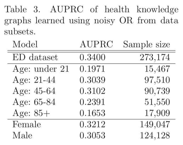
The lower AUPRC for older patients may also reflect their having more diseases.

Still, a larger sample is not necessarily better:

• “the number of occurrences [of a disease in the records] does not appear to be associated with high or low F1” (p. 25, but conflicts with p. 21? “diseases with lower performance correlate with... fewer observations”)
  
  
• using CR instead of ED does not give higher AUPRC (Table 5, next slide)

Data “Granularity”

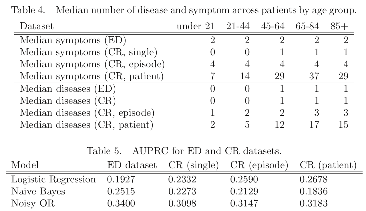
More aggregation helps LR but not NB, why? Authors: “likely due to violations in the conditional independence that NB assumes”

The best value is for NO/ED, their previous/original network. It makes sense that an ED record would be more likely to present the salient symptoms and diseases for a patient than a single chart note, and conversely that the aggregate record with more diseases per patient could make it harder to pair diseases with the “right” symptoms.

Potential Confounders and Model Limitations

• The more diseases a patient has, the more error:
  • symptoms may be difficult to attribute to the correct disease
  • one disease may increase the susceptibility to other diseases
  • multiple co-occurring diseases may be the result of an underlying problem
  
  
• The information gain with increasing aggregation (CR single → episode → patient) may overwhelm models like naive Bayes
  
  
• Diseases and symptoms in the gold standard GHKG were selected based on relevance to the acute emergency department environment. Authors: “The ED likely yields an adequate data set for most acute complaints... The CR dataset... may be biased towards more chronic conditions and symptoms.”
  
  
• The model assumes a bipartite graph of binary edges between diseases and symptoms; expanding this to other types of edges (e.g. disease causing another disease) may allow the health knowledge graph to better represent medical knowledge