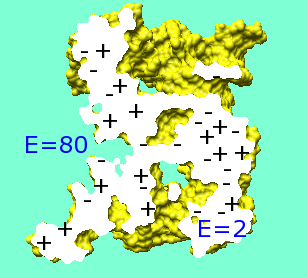
Typically, inside the molecular surface is assigned ε = 2-10 and outside is assigned ε = 78-80.
The Poisson equation is the fundamental equation of classical electrostatics:
∇2φ = (−4πρ)/εThat is, the curvature of the electrostatic potential (φ) at a point in space is directly proportional to the charge density (ρ) at that point and inversely proportional to the permittivity of the medium (ε). The permittivity or dielectric constant is the medium's responsiveness to charge and includes contributions from electronic polarization and the reorientation and movement of atoms. Higher ε corresponds to a greater responsiveness and greater ability to screen charges from other charges. In vacuum, ε = 1.
If all charges are represented explicitly, the Poisson equation simplifies to the Coulomb equation (and ε = 1 is generally used):
φ = (1/ε) Σ(qi/di)That is, the electrostatic potential at a point in space is a sum over the charges in the system scaled by their distances from that point. Because the response of the medium involves motion, however, simulations are required to model the system, for example, to allow water molecules to reorient around a charged solute.
If the solvent is represented by a continuum instead of explicitly, then it is necessary to solve the Poisson equation to get the spatial distribution of the electrostatic potential (what we show with Volume Viewer and Surface Color in Chimera) and the total electrostatic energy of the system:
electrostatic energy = (½) Σ(qiφi)With appropriate thermodynamic cycles, it is possible to calculate electrostatic contributions to solvation energy, binding energy, etc. However, most often the calculation is run for a single, static set of coordinates embedded in a high dielectric, to represent the molecule(s) in aqueous solution:
|
Major inputs:
coordinates, atomic radii, atomic point charges,
"inside" and "outside" dielectrics, ionic strength
(but be aware there are many other parameters)
Typically, inside the molecular surface is assigned ε = 2-10 and outside is assigned ε = 78-80. |
When ε is not a single constant over the whole system, the Poisson equation becomes
∇ · ε∇φ = −4πρand including mobile ions makes it the Poisson-Boltzmann equation
(why DelPhi is the best program name ever!!)
∇ · ε∇φ − (ions term) = −4πρwhich can be linearized under the assumption that φ is small relative to kT. The linearized form can be solved more rapidly.
For molecules of arbitrary shape (not a perfect sphere, for example), the equation has to be solved numerically rather than analytically. In finite-difference Poisson-Boltzmann (FDPB) calculations, space is gridded up and the equation is solved by finite difference iteration to convergence. Various algorithmic tricks are used to speed convergence. The finite-difference equation:
where φo is the potential at a particular grid point, φi is the potential at the six nearest neighbors, and εi is the dielectric constant at the midpoint between φo and φi. Essentially, the potential at a grid point keeps adjusting based on the potentials at the nearest neighbor grid points. In DelPhi, the potential comes out in units of kT/e.
φo = (Σεiφi) + (4πqo/grid-res) (Σεi) + (another ions term)o
Errors due to discretization are addressed by focussing (multiple runs with the molecule(s) filling successively larger portions of the box, to minimize errors due to boundary conditions) and averaging over calculations with shifted (rotated and/or translated) grid positions.
Electrostatic potential maps obtained from continuum electrostatic calculations can be very different than those obtained using Coulomb's equation with a constant or distance-dependent dielectric (ε = 4r is commonly used as the best, yet not very good, approximation when neither continuum dielectric nor explicit solvent calculations are feasible). The presence of different dielectric regions and their detailed shapes are important in determining the distribution of electrostatic potential.
The "force field scoring" I put in DOCK 3.0 allowed constant or distance-dependent dielectrics to be used, with ε = 4r recommended. Swiss-PdbViewer calculates a Coulombic potential (see documentation). So does Midas (esp command, apparently using parameter files of partial charges of atoms in standard residues).
Many programs perform numerical PB calculations, including:
Review of electrostatics equations and several different approaches to calculating electrostatics.
Relatively short overview of scientific applications of continuum electrostatic calculations (only one equation!).